Leadscrews are fundamental components in many mechanical systems. They convert rotational motion into linear motion and are widely used in precision instruments, manufacturing equipment, robotic mechanisms, and positioning systems. Understanding the dynamics of a leadscrew system is important for predicting system response, designing controllers, estimating required motor torque, and evaluating the influence of load, damping, stiffness, and transmission efficiency.

In this post, we examine a simplified mathematical model of a leadscrew-driven translational system. The goal is to derive equations of motion that relate the applied motor torque to the resulting linear motion of the load.

The model assumes forward-driving operation, where motor torque drives the screw and produces linear motion of the load. Direction-dependent friction, backlash, compliance of the screw/nut interface, and nonlinear friction effects are neglected unless they are explicitly represented through an efficiency factor.

I. Key Parameters

Before deriving the equations, we define the key parameters used in the leadscrew system.

Parameter	Definition	Explanation	Unit
\(J\)	Moment of inertia of the screw and rotating components	Resistance of the rotating components to angular acceleration	\(kg\,m^2\)
\(B_r\)	Rotational damping coefficient	Viscous energy loss in rotational motion	\(N\,m\,s/rad\)
\(\theta\)	Angular displacement of the screw	Rotation angle of the screw	\(rad\)
\(T\)	Applied motor torque	Torque applied to the screw	\(N\,m\)
\(T_{\text{load}}\)	Equivalent load torque reflected to the screw	Torque required at the screw to generate the axial load force	\(N\,m\)
\(m\)	Mass of the load	Translational mass driven by the leadscrew	\(kg\)
\(b_t\)	Translational damping coefficient	Viscous energy loss in linear motion	\(N\,s/m\)
\(k\)	Translational stiffness	Equivalent stiffness acting on the load	\(N/m\)
\(x\)	Linear displacement of the load	Translational displacement of the load	\(m\)
\(F\)	Axial force on the load	Force transmitted to the load through the leadscrew	\(N\)
\(p\)	Pitch of the leadscrew	Linear travel per full revolution	\(m/rev\)
\(\eta\)	Forward-driving efficiency of the leadscrew	Ratio of useful linear output work to rotational input work	Dimensionless

II. Equations

We first write the rotational and translational equations separately, then connect them using the kinematic relationship between screw rotation and load displacement.

1. Rotational Equation of Motion

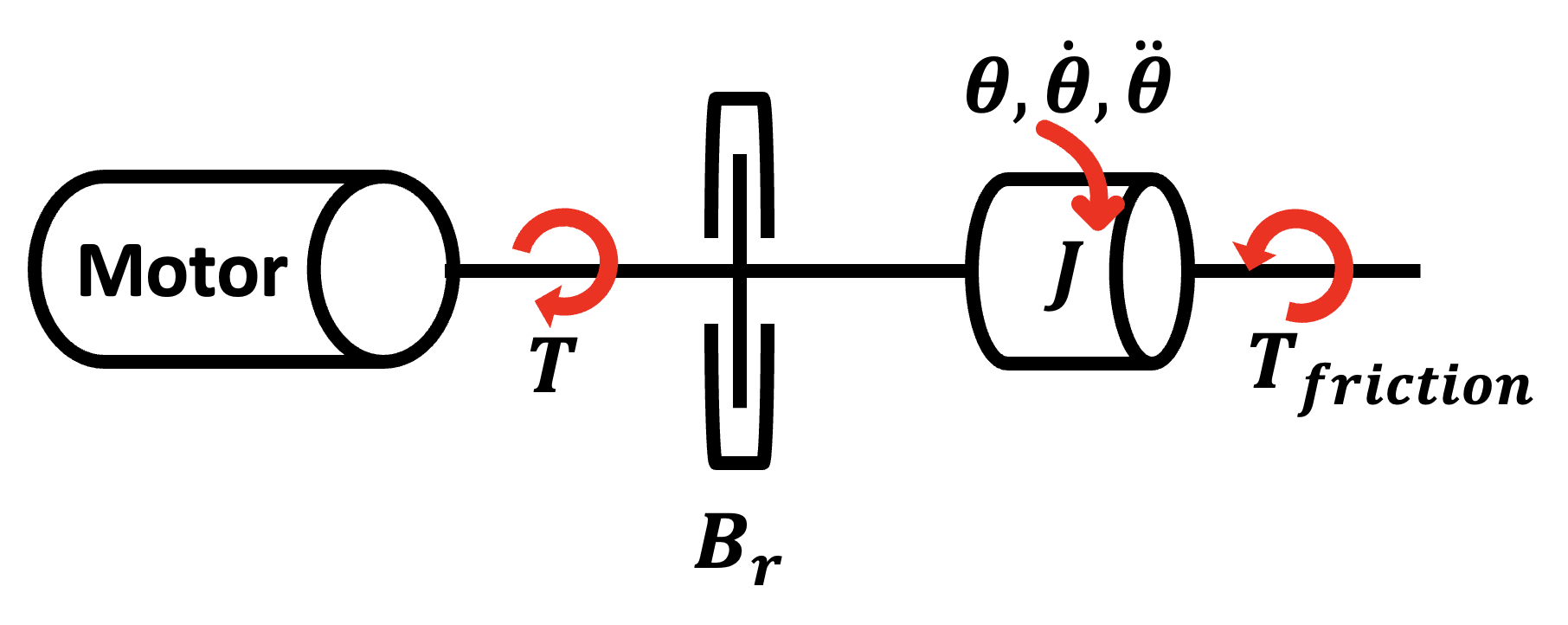
The rotational dynamics of the screw can be written as

\begin{equation} J\ddot{\theta} + Br\dot{\theta} + T{\text{load}} = T \label{eq:rotational_eom} \end{equation}

where \(\ddot{\theta}\) is the angular acceleration, \(\dot{\theta}\) is the angular velocity, and \(T_{\text{load}}\) is the equivalent torque required to drive the axial load through the leadscrew.

For a forward-driving leadscrew, the useful linear work over one revolution is

\begin{equation} W_{\text{out}} = Fp \label{eq:output_work} \end{equation}

and the rotational input work is

\begin{equation} W{\text{in}} = T{\text{load}}(2\pi) \label{eq:input_work} \end{equation}

Using the efficiency definition

\begin{equation} \eta = \frac{W{\text{out}}}{W{\text{in}}} \label{eq:efficiency_definition} \end{equation}

we obtain

\begin{equation} T_{\text{load}} = \frac{Fp}{2\pi\eta} \label{eq:equivalent_load_torque} \end{equation}

This term is not purely a friction torque. It is the equivalent input torque required to generate the axial force \(F\) while accounting for transmission efficiency.

2. Translational Equation of Motion

The linear motion of the load is described by

\begin{equation} m\ddot{x} + b_t\dot{x} + kx = F \label{eq:translational_eom} \end{equation}

where \(\ddot{x}\) is the linear acceleration, \(\dot{x}\) is the linear velocity, and \(kx\) is the restoring force due to the equivalent translational stiffness.

3. Relationship Between Rotational and Translational Motion

The leadscrew kinematic relationship is

\begin{equation} x = \frac{p\theta}{2\pi}, \qquad \dot{x} = \frac{p\dot{\theta}}{2\pi}, \qquad \ddot{x} = \frac{p\ddot{\theta}}{2\pi} \label{eq:kinematic_relation} \end{equation}

Equivalently,

\begin{equation} \theta = \frac{2\pi}{p}x, \qquad \dot{\theta} = \frac{2\pi}{p}\dot{x}, \qquad \ddot{\theta} = \frac{2\pi}{p}\ddot{x} \label{eq:inverse_kinematic_relation} \end{equation}

III. Combined Equation of Motion

We now combine the rotational and translational dynamics to obtain a single equation of motion.

1. In Terms of Angular Displacement (\(\theta\))

Using \eqref{eq:translational_eom} and the kinematic relationship in \eqref{eq:kinematic_relation}, the axial force can be written as

\begin{equation} F = \frac{p}{2\pi} \left( m\ddot{\theta}

• b_t\dot{\theta}
• k\theta \right) \label{eq:force_theta_domain} \end{equation}

Substituting \eqref{eq:force_theta_domain} into \eqref{eq:equivalent_load_torque} gives

\begin{equation} T_{\text{load}} = \frac{p^2}{(2\pi)^2\eta} \left( m\ddot{\theta}

• b_t\dot{\theta}
• k\theta \right) \end{equation}

Substituting this result into \eqref{eq:rotational_eom} yields

\begin{equation} \left( J + \frac{mp^2}{(2\pi)^2\eta} \right)\ddot{\theta}

• \left( B_r + \frac{b_t p^2}{(2\pi)^2\eta} \right)\dot{\theta}

• \frac{k p^2}{(2\pi)^2\eta}\theta

  T \label{eq:combined_rotational_domain} \end{equation}

Equation \eqref{eq:combined_rotational_domain} expresses the leadscrew-driven system in the rotational domain. The translational mass, damping, and stiffness are reflected to the screw side through the factor \(p^2/(2\pi)^2\eta\).

2. In Terms of Linear Displacement (\(x\))

Using the inverse kinematic relationship in \eqref{eq:inverse_kinematic_relation}, Eq. \eqref{eq:combined_rotational_domain} becomes

\begin{equation} \left( J + \frac{mp^2}{(2\pi)^2\eta} \right) \frac{2\pi}{p}\ddot{x}

• \left( B_r + \frac{b_t p^2}{(2\pi)^2\eta} \right) \frac{2\pi}{p}\dot{x}
• \frac{k p^2}{(2\pi)^2\eta} \frac{2\pi}{p}x = T \label{eq:substituted_linear_domain} \end{equation}

Multiplying both sides of \eqref{eq:substituted_linear_domain} by \(2\pi\eta/p\) yields

\begin{equation} \left( m + \frac{(2\pi)^2\eta J}{p^2} \right)\ddot{x}

• \left( b_t + \frac{(2\pi)^2\eta B_r}{p^2} \right)\dot{x}

• kx

  \frac{2\pi\eta}{p}T \label{eq:combined_linear_domain} \end{equation}

The coefficients in Eq. \eqref{eq:combined_linear_domain} correspond to the equivalent mass and damping reflected to the translational domain.

Therefore, the equivalent linear parameters are

\begin{equation} m_{\text{eq}} = m + \frac{(2\pi)^2\eta J}{p^2} \label{eq:equivalent_mass} \end{equation}

\begin{equation} b_{\text{eq}} = b_t + \frac{(2\pi)^2\eta B_r}{p^2} \label{eq:equivalent_damping} \end{equation}

and

\begin{equation} F_{\text{input}} = \frac{2\pi\eta}{p}T \label{eq:equivalent_input_force} \end{equation}

Thus, Eq. \eqref{eq:combined_linear_domain} can be written compactly as

\begin{equation} m_{\text{eq}}\ddot{x}

• b_{\text{eq}}\dot{x}

• kx

  F_{\text{input}} \label{eq:compact_linear_domain} \end{equation}

IV. Remarks on Efficiency and Model Limitations

The equations above use a single constant efficiency \(\eta\). This is a simplified representation of losses in the leadscrew transmission. In real leadscrew systems, friction may depend on load direction, speed, lubrication, preload, wear, and whether the system is forward-driving or backdriving.

Therefore, the model should be interpreted as a simplified dynamic model suitable for basic system analysis and controller design. For high-fidelity modeling, additional effects such as Coulomb friction, Stribeck friction, backlash, screw compliance, nut compliance, and direction-dependent efficiency may need to be included.