[Controller Design] Day 2: PID Controller
I. Introduction
A fully actuated system is one in which the number of independent actuators matches the number of degrees of freedom, allowing for direct control over each motion dimension. This setup is typical in industrial robots and other motor-driven mechanisms, where each joint or axis is controlled by its own motor, facilitating precise manipulation.
In fully actuated multi-link mechanisms, each degree of freedom—whether it involves rotation or translation—is directly managed by an independent actuator. This direct manipulation allows for precise adjustments to the mechanism’s position and motion, simplifying the control algorithms needed for maintaining stability and achieving desired behaviors. While an understanding of nonlinear dynamics is beneficial for optimizing performance and handling complex scenarios, linear controllers often suffice for basic control tasks in these systems.
Today, we will focus on simulating the PID (Proportional-Integral-Derivative) controller, which is one of the simplest and most representative types of linear controllers. Figure 0 presents the block diagram of the PID controller system.
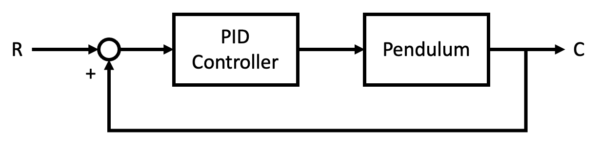
1. Principles of PID Control
PID control operates on three basic principles:
- Proportional (P): Applies correction proportional to the current error.
- Integral (we): Accumulates past errors to eliminate steady-state error.
- Derivative (D): Anticipates future errors based on the rate of change.
The control law can be expressed as:
\[u(t) = K_p e(t) + K_i \int_0^t e(\tau) d\tau + K_d \frac{de(t)}{dt} \tag{1}\]Where $u(t)$ is the control signal, $e(t)$ is the error, and \(K_p\), \(K_i\), and \(K_d\) are the proportional, integral, and derivative gains respectively.
2. Advantages and Limitations
Advantages:
- Simple design and implementation
- Effective for a wide range of linear systems
- Can be tuned intuitively without detailed system models
Limitations:
- May struggle with highly nonlinear systems
- Potential for integral windup in systems with actuator saturation
- Derivative term can amplify noise in the system
3. Applications
PID controllers find wide application in various fields:
- Industrial processes: Temperature, pressure, and flow control
- Robotics: Joint position and velocity control
- Automotive systems: Cruise control, anti-lock braking systems
- Aerospace: Attitude control in satellites and aircraft
- Consumer electronics: Speed control in disk drives
4. Stability Considerations
The stability of a PID-controlled system depends on proper tuning of the gains \(K_p\), \(K_i\), and \(K_d\). Various methods exist for tuning these parameters, including:
- Ziegler-Nichols method
- Cohen-Coon method
- Iterative tuning based on step response characteristics
Stability analysis often involves techniques such as root locus plots or frequency response methods to ensure the closed-loop system remains stable across its operating range.
In the following sections, we will delve deeper into the implementation and simulation of a PID controller for a multi-link mechanism, exploring its performance characteristics and discussing tuning strategies.
II. A Multi-Link Mechanism with a Fixed Base
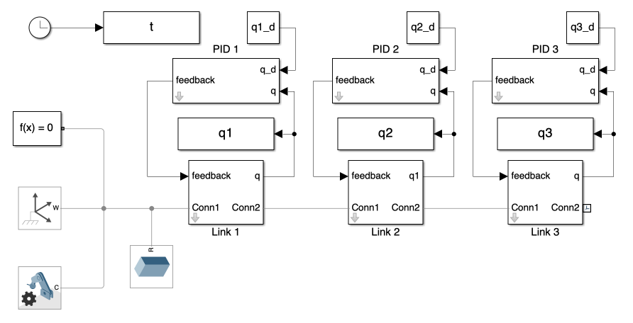
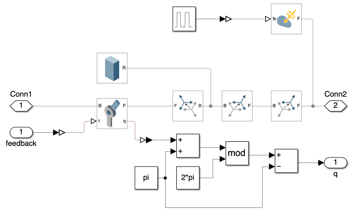
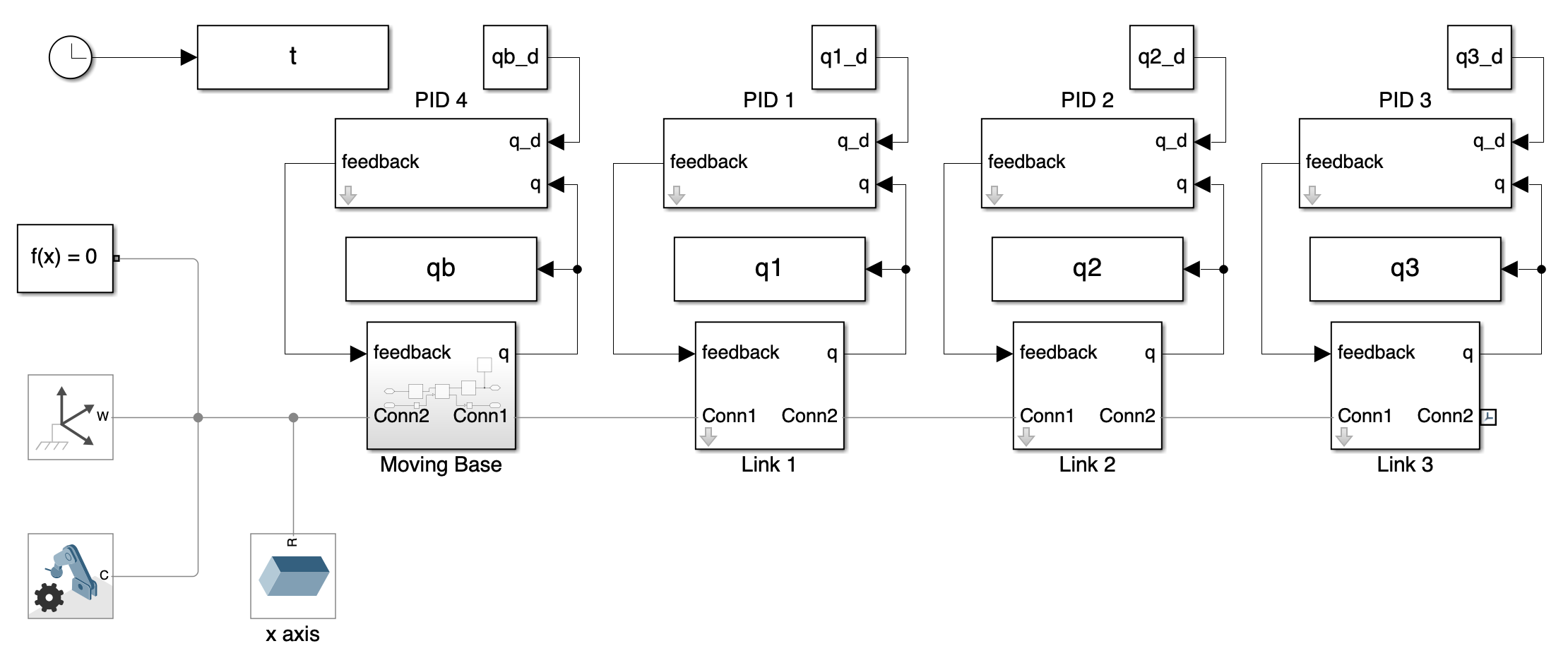
1. Overall System
The overall system is depicted in Figure 1. This system closely resembles that of Day 1 but includes an added PID control subsystem. The angular displacement of each joint is input into the PID controller block, which calculates the feedback torque to actuate the joints.
2. Subsystems
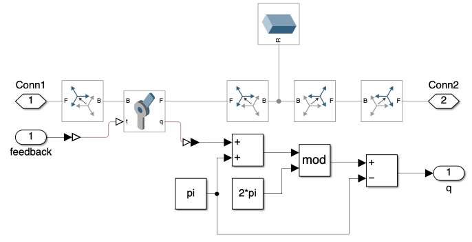
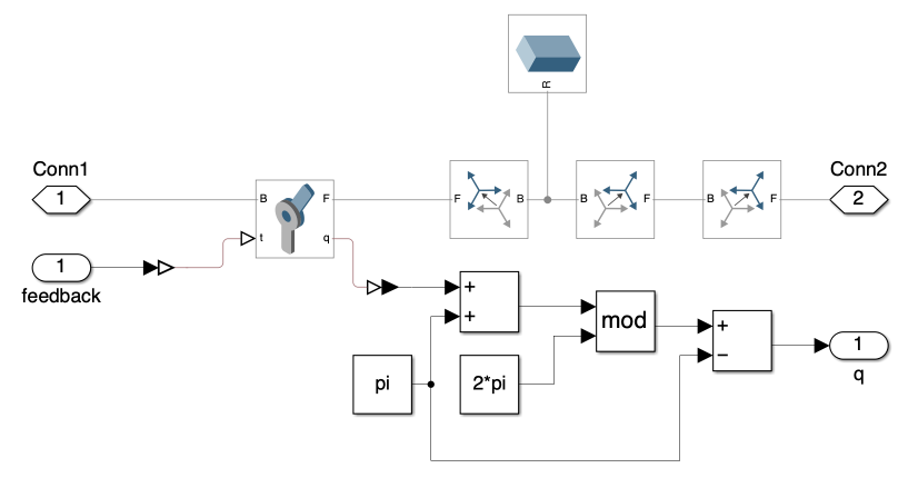
1) Links
In the updated design of the link subsystems, illustrated in Figures 2, 3, and 4, we’ve introduced several modifications to enhance realism and functionality. These changes echo the foundational setups from Day 1 but with key differences:
- To better realize the oscillatory nature of real-world multi-link mechanism dynamics, we’ve configured the angular displacement of each link to be periodic, spanning a full circle from \(-\pi\) to \(\pi\).
- In a shift from the initial configuration, we’ve realigned the x-axis of link 1 to coincide with the z-axis of the world frame.
- Additionally, we’ve incorporated blocks to generate an impulsive external force at the end of link 3, to simulate external forces on the system and test its regulatory response.
The modifications ensure that when the multi-link mechanism is upright, its angular displacement is set to \(0\). This allows us to use the origin as our equilibrium point in subsequent simulations.
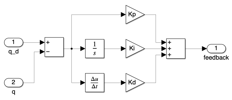
2) PID Controller
Figure 5 shows a PID controller subsystem. It begins by comparing a desired target (q_d) with an actual value (q) to determine the error, or the difference between what is desired and what exists. This error is then processed through three types of control: Proportional (Kp), which reacts to the current error; Integral (Ki), which addresses the accumulation of past errors; and Derivative (Kd), which predicts future errors. The outputs from these controls are combined to produce a feedback signal that adjusts the system to minimize the error, helping maintain the desired output.
3. Simulation
In this section, we explore the simulation, focusing on both tracking and regulation capabilities of the system with fixed base. Through these simulations, we aim to validate the effectiveness of the controllers in maintaining trajectory accuracy (tracking) and stabilizing the system against disturbances (regulation).
1) Tracking
Videos 1 through 4 demonstrate the behavior of the system from various initial states. Figures 6 through 9 present an analysis of angular displacement for different initial conditions. These results show the robust tracking capabilities of the control system, which efficiently elevates the multi-link mechanism to a vertical position from any initial state.
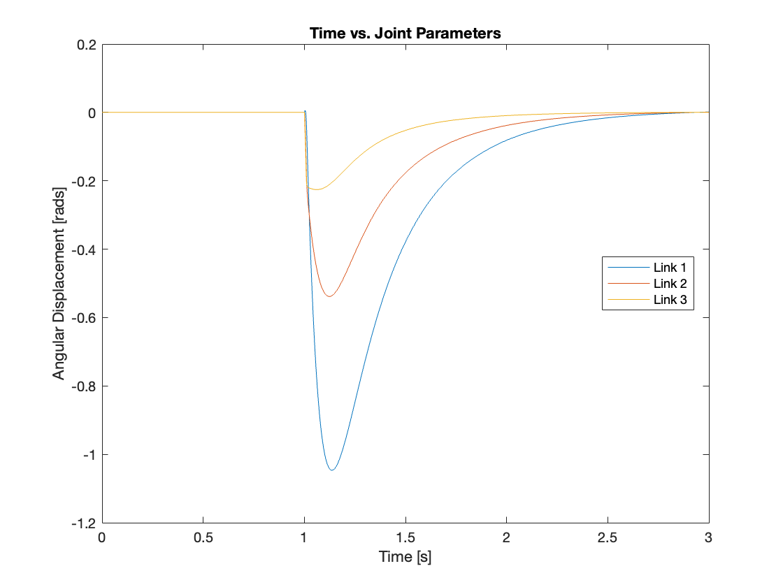
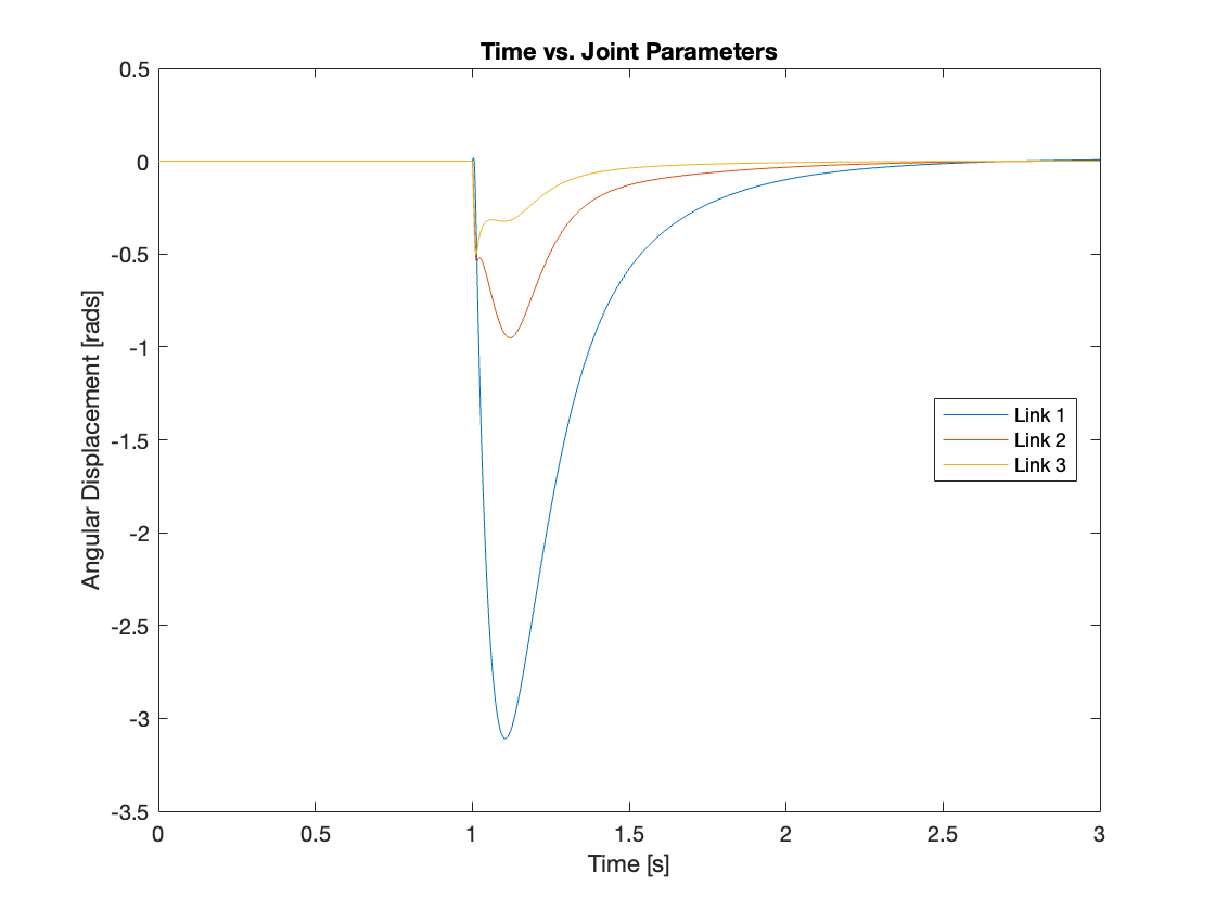
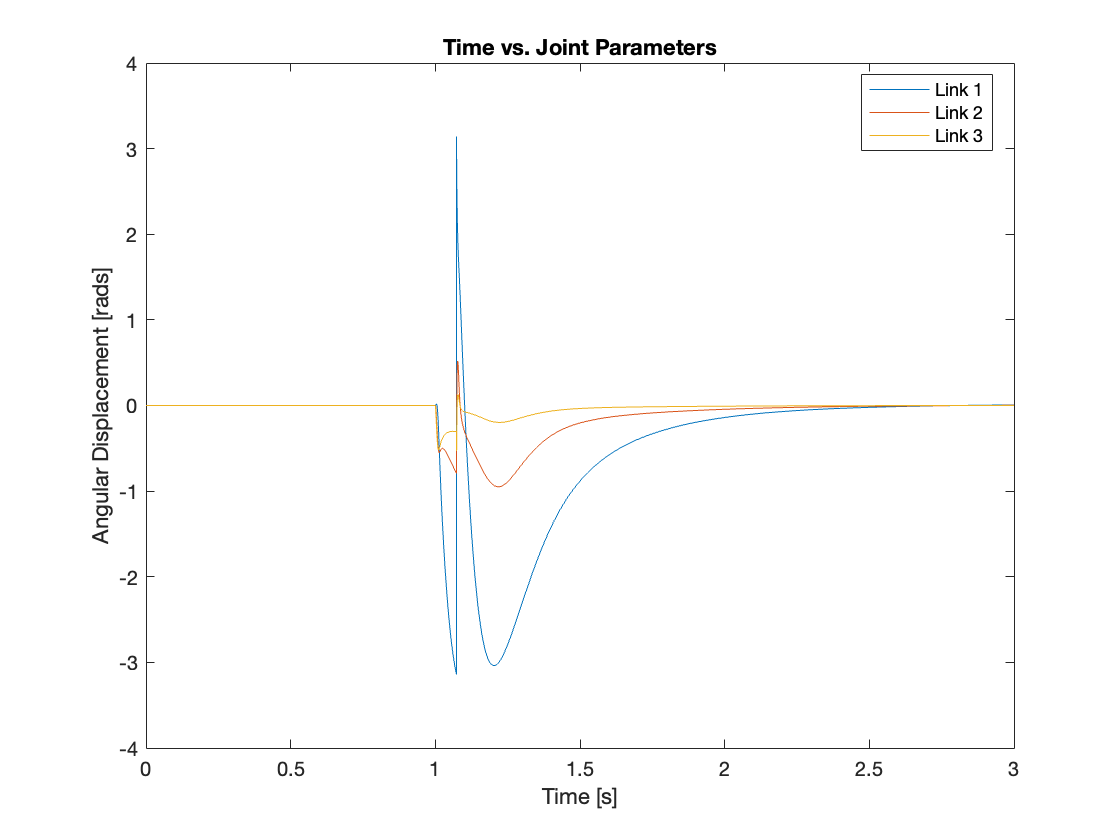
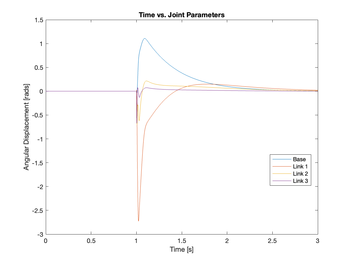
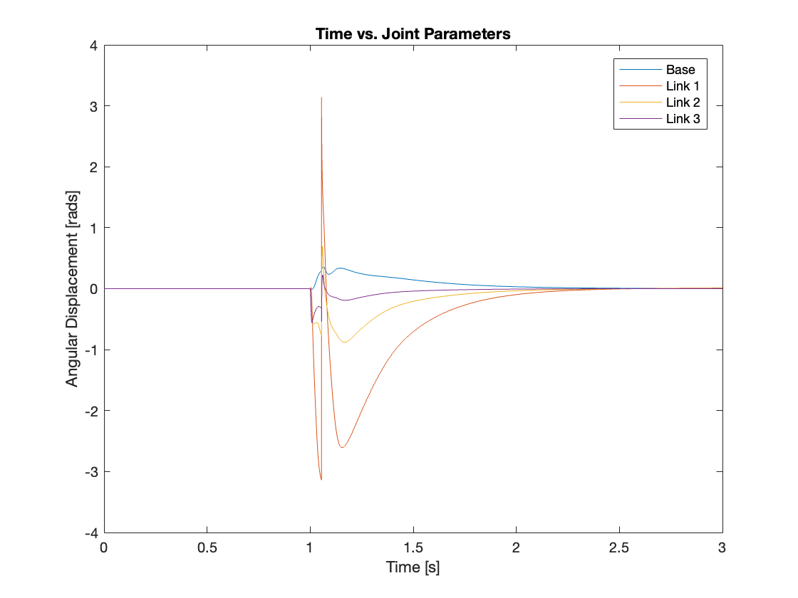
2) Regulation
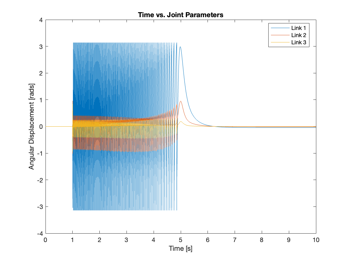
Videos 5 through 9 demonstrate the robust regulating capabilities of the control system, which efficiently rejects disturbances and maintains the reference position. Meanwhile, Figures 6 through 9 analyze the angular displacement under various disturbances. Specifically, Videos 6 and 7, along with Figures 11 and 12, showcase a simulation of a triple-link mechanism subjected to a substantial disturbance, significant enough to potentially cause a single rotation. However, in these demonstrations, the multi-link mechanism rotates almost twice. Similarly, As demonstrated in Video 8 and Figure 13, the system exhibits prolonged regulation times when subjected to a strong disturbance. We suspect this excessive rotation is due to the control system not accounting for the angular velocity and angular acceleration of the multi-link mechanism. This oversight in the control strategy leads to an over-response to the disturbance. We am uncertain whether this issue can be addressed by tuning the PID controller or changing system parameters. Please leave a comment if you have any ideas.
III. A Multi-Link Mechanism with a Moving Base
1. Overall System
The overall system configuration of the triple-link mechanism with a moving base is similar to that of the fixed base, with the addition of a moving frame. Also, we have increased the density of the base to make it heavier.
2. Simulation
In this section, we explore the simulation, focusing on both tracking and regulation capabilities of the system with moving base. Through these simulations, we aim to validate the effectiveness of the controllers in maintaining trajectory accuracy (tracking) and stabilizing the system against disturbances (regulation).
1) Tracking
Videos 9 through 12 showcase the robust tracking capabilities of the control system, which efficiently brings the multi-link mechanism to a vertical position from any starting point. Meanwhile, Figures 15 through 18 provide an analysis of angular displacement across various initial states. Interestingly, the trajectory of the system with a moving base appears more sensible than that of the system with a fixed base, likely due to the addition of an extra degree of freedom.
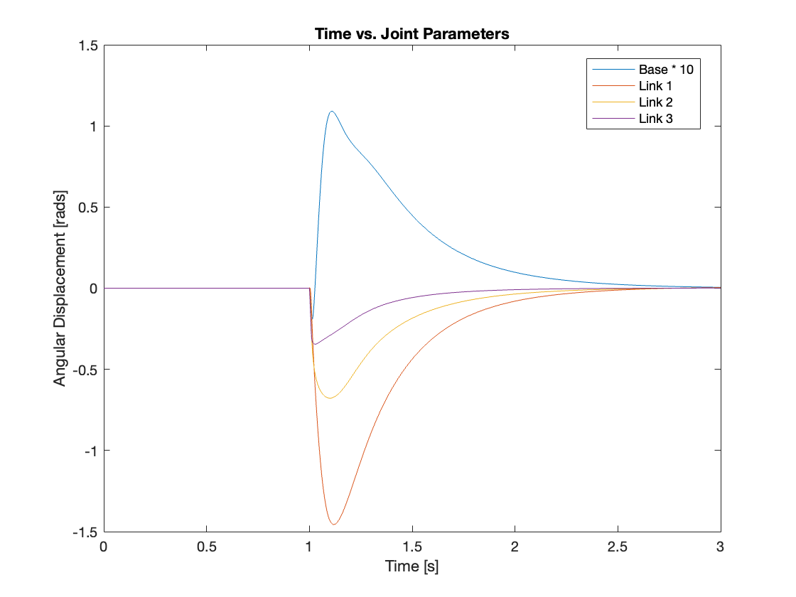
2) Regulation
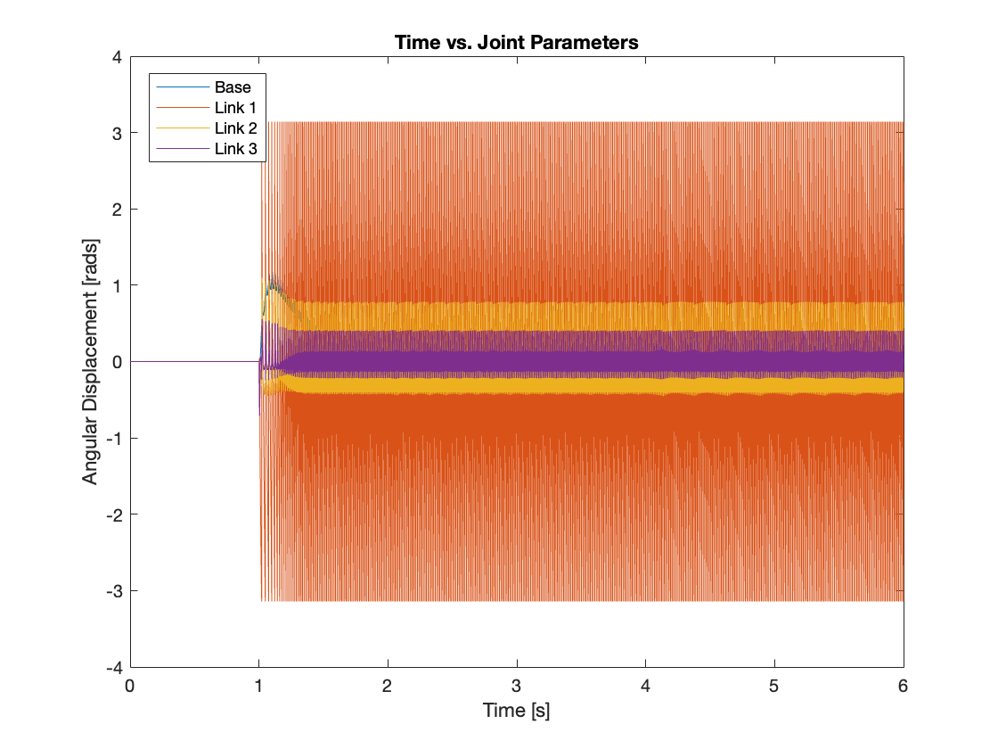
Videos 13 through 16 illustrate the regulating capabilities of the control system, which effectively rejects disturbances and maintains the reference position in most scenarios. Meanwhile, Figures 19 through 22 provide an analysis of angular displacement under various disturbances.
Specifically, Videos 13 to 15 demonstrate conditions with low base density under mild and strong disturbances, and very high base density under strong disturbance, respectively. Under these setups, the system regulates effectively, either by the base dispersing the energy or functioning as a fixed base. However, as shown in Video 16, under certain combinations of base density and disturbance intensity, the regulation is not successful, and the system becomes unstable. This instability is likely because, similar to the fixed base scenario, the PID controller primarily considers angular displacement, which may not suffice under more challenging conditions.
IV. Conclusion and Moving Forward
Today, we dealt with a fully actuated multi-link mechanism using a PID controller. This control system offers the benefit of a relatively simple design, as it does not require consideration of the complete dynamic equations of the triple-link mechanism. However, this simplicity sometimes leads to drawbacks, such as overreaction or subsequent destabilization of the system. In our next post, we will explore alternative control systems that can address these issues. Stay tuned for more updates as we delve deeper into the intriguing world of multi-link mechanisms and confront the challenges of controlling chaotic systems!
You can find the Simulink model on my GitHub repository.
Enjoy Reading This Article?
Here are some more articles you might like to read next: