In our previous work, we implemented a PID controller that relied solely on the difference between the reference angle and the current angle. Due to its simplistic mechanism, an in-depth understanding of the triple-link mechanism’s behavior was not required. However, given the inherent nonlinearity of the triple-link mechanism, the PID controller proved somewhat inefficient and performed less effectively compared to other controllers.

Subsequent controllers necessitate a thorough analysis of the triple-link mechanism’s behavior. Therefore, we will explore the equations of motion and the Jacobians of the triple-link mechanism in detail.

I. Introduction

Lagrangian dynamics offers a powerful and flexible approach to analyzing complex mechanical systems, such as multi-link mechanisms. This method provides a systematic way to derive equations of motion and understand system behavior, which is crucial for effective control design.

1. Lagrangian Dynamics

Lagrangian dynamics, in contrast to Newtonian dynamics, allows the use of any set of variables—known as generalized coordinates, denoted q—as long as they uniquely describe the position of the bodies within the system. The core of this approach is the Lagrangian, defined as:

\[L = KE - PE \tag{1}\]

Where \(KE\) represents the total kinetic energy of the system, and \(PE\) denotes the total potential energy, both expressed in terms of generalized coordinates (e.g., \(x, \theta_1\)).

The equations of motion are derived using the following relationship:

\[\left(\frac{d}{dt}\frac{\partial L}{\partial \dot{q}} - \frac{\partial L}{\partial q}\right)^T = Q \tag{2}\]

Here, \(Q\) is a vector that includes each of the generalized forces associated with the chosen generalized coordinates (e.g., \(f_x, \tau_1\)).

2. Equations of Motion for Multi-Link Mechanisms

Using Lagrangian dynamics, we can derive the equation of motion for a multi-link mechanism. For instance, the equation of motion for a double-link mechanism is:

\[\begin{bmatrix}\tau_1 \\ \tau_2 \end{bmatrix} = \begin{bmatrix} M_{1, 1} & M_{1, 2} \\ M_{2, 1} & M_{2, 2} \end{bmatrix}\begin{bmatrix}\ddot{\theta}_1 \\ \ddot{\theta}_2 \end{bmatrix} + \begin{bmatrix} h_{1, 1}\dot{\theta}_2^2 + h_{1, 2}\dot{\theta}_1\dot{\theta}_2 \\ h_{2, 1}\dot{\theta}_1^2 \end{bmatrix} + \begin{bmatrix} g_{1} \\ g_{2}\end{bmatrix}g \tag{3}\]

Where:

• Matrix M (Inertial Term): Represents the Newtonian response of the system to applied forces, accounting for the inertia of the masses.
• Matrix h (Coriolis and Centrifugal Forces):
  • Centrifugal Force: Arises from terms like \(\dot{\theta}_1^2, \dot{\theta}_2^2\) and affects the system when rotating.
  • Coriolis Force: Results from terms like \(\dot{\theta}_1\dot{\theta}_2\) and is evident when components of the system move relative to one another.
• Matrix g (Gravitational Term): Accounts for the force due to gravity acting on each mass component.

3. Jacobian Matrices in Robotics

The Jacobian matrix is a fundamental tool in linear approximation, playing a crucial role in understanding how small changes in input variables affect output variables. For a function \(\mathbf{f}\) that maps inputs \(\mathbf{q} = (q_1, q_2, ..., q_n)\) in \(\mathbb{R}^n\) to outputs \(\mathbf{p} = (p_1, p_2, ..., p_m)\) in \(\mathbb{R}^m\), the Jacobian matrix \(\mathbf{J}\) is given by:

\[\mathbf{J} = \begin{bmatrix} \frac{\partial p_1}{\partial q_1} & \frac{\partial p_1}{\partial q_2} & \cdots & \frac{\partial p_1}{\partial q_n} \\ \frac{\partial p_2}{\partial q_1} & \frac{\partial p_2}{\partial q_2} & \cdots & \frac{\partial p_2}{\partial q_n} \\ \vdots & \vdots & \ddots & \vdots \\ \frac{\partial p_m}{\partial q_1} & \frac{\partial p_m}{\partial q_2} & \cdots & \frac{\partial p_m}{\partial q_n} \end{bmatrix} \tag{4}\]

In the context of multi-link mechanisms, the Jacobian matrix captures the relationship between joint parameters and the position and orientation of the end-effector or, in some cases, the center of mass of the final link.

These principles form the foundation for understanding and controlling complex mechanical systems, enabling the development of sophisticated control strategies for multi-link mechanisms.

II. Our Scenario

A. A Triple-Link Mechanism with a Fixed Base

The free body diagram of the triple-link mechanism with a fixed base is illustrated in Figure 1. In this diagram, the positive z-axis of the global frame is initially considered as the reference position. For simplification purposes, we have designated the x-axis of the global frame as the new reference position, leading to the relationship \(\theta_1 = \frac{\pi}{2} + q_1\). The variables \(q_2\) and \(q_3\) are retained as \(\theta_2\) and \(\theta_3\), respectively.

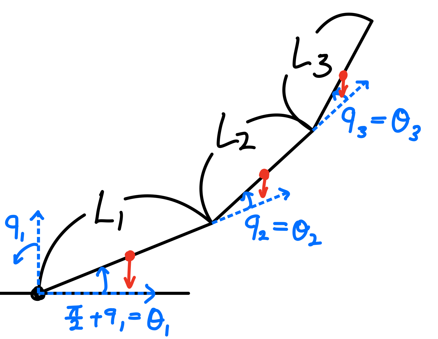
• \(\theta_i\): the joint angle of joint \(i\)
• \(m_i\): the mass of link \(i\)
• \(I_i\): the moment of inertia of link \(i\) about the axis that passes through the center of mass and is parallel to the \(Z_i\)-axis
• \(l_i\): the length of link \(i\)
• \(g\): the magnitude of gravitational acceleration
• \(S_{ijk}\): \(\sin(\theta_i + \theta_j + \theta_k)\)
• \(C_{ijk}\): \(\cos(\theta_i + \theta_j + \theta_k)\)

The moment of inertia for each link in our system can be calculated using the formula:

\[we = \frac{1}{12}m(l^2 + w^2) \approx \frac{1}{12}ml^2\]

This approximation holds because the length \(l\) of each link significantly exceeds its width \(w\). Given this, we can describe the center of mass for each link as follows:

• For the link 1: \(s_1 = \begin{bmatrix} \frac{1}{2} l_1 \cos(\theta_1) \\ \frac{1}{2} l_1 \sin(\theta_1) \end{bmatrix}\)
• For the link 2: \(s_2 = \begin{bmatrix} l_1 \cos(\theta_1) + \frac{1}{2} l_2 \cos(\theta_{12}) \\ l_1 \sin(\theta_1) + \frac{1}{2} l_2 \sin(\theta_{12}) \end{bmatrix}\)
• For the link 3: \(s_3 = \begin{bmatrix} l_1 \cos(\theta_1) + l_2 \cos(\theta_{12}) + \frac{1}{2} l_3 \cos(\theta_{123}) \\ l_1 \sin(\theta_1) + l_2 \sin(\theta_{12}) + \frac{1}{2} l_3 \sin(\theta_{123}) \end{bmatrix}\)

1) Equation of Motion

The linear velocity of each link’s center of mass is expressed as:

\[\dot{s} = \frac{ds}{dt}.\]

Similarly, the angular velocity for each link is summed up to:

\[\sum_{k=1}^i \dot{\theta}_k.\]

The energy dynamics of the system are defined by the kinetic and potential energies:

\[KE_i = \frac{1}{2} m_i \dot{s}_i^\top \dot{s}_i + \frac{1}{2} I_i \left( \sum_{k=1}^i \dot{\theta}_k \right)^2,\] \[PE_i = m_i g s_{i, 2},\]

where \(s_{i, 2}\) represents the y-component of the vector \(s_i\).

The overall dynamics are governed by the Lagrangian, which is:

\[L = \sum_{i=1}^3 KE_i - \sum_{i=1}^3 PE_i.\]

Finally, by substituting \(L\) into equation (1), we derive the equations of motion. We will not detail the derivation and results here due to their length.

2) Jacobian

The position and orientation of the center of mass of link 3 are represented as follows:

\[\mathbf{f} = \begin{bmatrix} x_{g, 3} \\ y_{g, 3} \\ \Omega \end{bmatrix} = \begin{bmatrix} l_1 \cos(\theta_1) + l_2 \cos(\theta_{12}) + \frac{1}{2} l_3 \cos(\theta_{123}) \\ l_1 \sin(\theta_1) + l_2 \sin(\theta_{12}) + \frac{1}{2} l_3 \sin(\theta_{123}) \\ \theta_1 + \theta_2 + \theta_3 \end{bmatrix}\]

Consequently, the Jacobian matrix is given by:

\[J = \begin{bmatrix} \frac{\partial x_{g, 3}}{\partial \theta_1} & \frac{\partial x_{g, 3}}{\partial \theta_2} & \frac{\partial x_{g, 3}}{\partial \theta_3} \\ \frac{\partial y_{g, 3}}{\partial \theta_1} & \frac{\partial y_{g, 3}}{\partial \theta_2} & \frac{\partial y_{g, 3}}{\partial \theta_3} \\ 1 & 1 & 1 \end{bmatrix}\]

where:

• \(x_{g, 3}\) and \(y_{g, 3}\) are the \(x\) and \(y\) coordinates of the center of mass of link 3.
• The derivatives \(\frac{\partial x_{g, 3}}{\partial \theta_i}\) and \(\frac{\partial y_{g, 3}}{\partial \theta_i}\) involve sine and cosine functions reflecting changes in position with respect to changes in the angles \(\theta_1\), \(\theta_2\), and \(\theta_3\).
• The third row reflects the direct additive impact of each joint angle on the overall orientation \(\Omega\).

For the complete calculations and results, please refer to the ‘Day_03_Fixed_Base.m’ file available on GitHub repository.

B. A Triple-Link Mechanism with a Moving Base

The free body diagram of the triple-link mechanism with a moving base is illustrated in Figure 2. It is similar to the fixed base but we added another parameter (\(x\)).

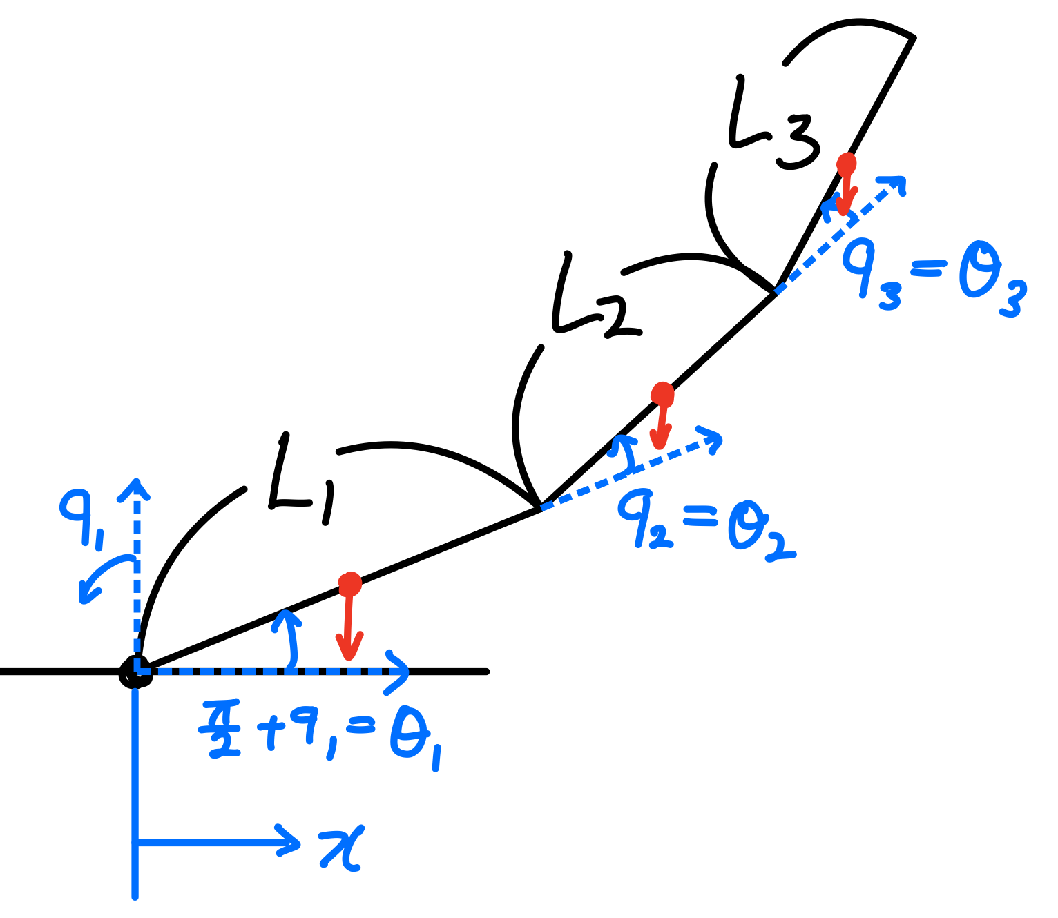
Since \(x\) influences the x-component of each center of mass, we must update them accordingly.

• For the base: \(s_0 = \begin{bmatrix} x \\ 0 \end{bmatrix}\)
• For the link 1: \(s_1 = \begin{bmatrix} x + \frac{1}{2} l_1 \cos(\theta_1) \\ \frac{1}{2} l_1 \sin(\theta_1) \end{bmatrix}\)
• For the link 2: \(s_2 = \begin{bmatrix} x + l_1 \cos(\theta_1) + \frac{1}{2} l_2 \cos(\theta_{12}) \\ l_1 \sin(\theta_1) + \frac{1}{2} l_2 \sin(\theta_{12}) \end{bmatrix}\)
• For the link 3: \(s_3 = \begin{bmatrix} x + l_1 \cos(\theta_1) + l_2 \cos(\theta_{12}) + \frac{1}{2} l_3 \cos(\theta_{123}) \\ l_1 \sin(\theta_1) + l_2 \sin(\theta_{12}) + \frac{1}{2} l_3 \sin(\theta_{123}) \end{bmatrix}\)

1) Equation of Motion

The approach remains the same as with the fixed base. However, we needed to account for the fact that there is only translational motion in the base.

\[L = \sum_{i=0}^3 KE_i - \sum_{i=0}^3 PE_i.\]

2) Jacobian

The function \(f\) f remains unchanged, but we must update the Jacobian matrix \(J\) as follows:

\[J = \begin{bmatrix} 1 & \frac{\partial x*{g, 3}}{\partial \theta*1} & \frac{\partial x*{g, 3}}{\partial \theta*2} & \frac{\partial x*{g, 3}}{\partial \theta*3} \\ 0 & \frac{\partial y*{g, 3}}{\partial \theta_1} & \frac{\partial y*{g, 3}}{\partial \theta*2} & \frac{\partial y*{g, 3}}{\partial \theta_3} \\ 0 & 1 & 1 & 1 \end{bmatrix}\]

For the complete calculations and results, please refer to the ‘Day_03_Moving_Base.m’ file available on GitHub repository.

C. A Pendulum on Cart

For a simplified model derived from the triple-link mechanism on a moving base, consider only the base and the first link.

• Base coordinates: \(s_0 = \begin{bmatrix} x \\ 0 \end{bmatrix}\)
• Link 1 coordinates: \(s_1 = \begin{bmatrix} x + \frac{1}{2} l_1 \cos(\theta_1) \\ \frac{1}{2} l_1 \sin(\theta_1) \end{bmatrix}\)

1) Equations of Motion:

The equations of motion for the system, including both inertial and gravitational effects, can be represented in matrix form as follows:

\[\begin{bmatrix} m_0 + m_1 & -\frac{m_1 l_1 \sin(\theta_1)}{2} \\ -\frac{l_1 m_1 \sin(\theta_1)}{2} & \frac{l_1^2 m_1}{3} \end{bmatrix} \begin{bmatrix} \ddot{x} \\ \ddot{\theta}_1 \end{bmatrix} + \begin{bmatrix} -\frac{1}{2}m_1 l_1 \cos(\theta_1) \dot{\theta}_1^2 \\ 0 \end{bmatrix} + \begin{bmatrix} 0 \\ \frac{1}{2}g l_1 m_1 \cos(\theta_1) \end{bmatrix} = \begin{bmatrix} F \\ 0 \end{bmatrix}\]

These equations of motion may appear unconventional because the angle reference \(\theta_1\) is defined from the horizontal (positive x-axis), rather than the more typical vertical reference. This orientation alters the trigonometric components and their interactions within the dynamic model, influencing how terms involving \(\sin(\theta_1)\) and \(\cos(\theta_1)\) are applied in the system’s matrix representation.

III. Conclusion

Today, we derived the equations of motion for a triple-link mechanism with both fixed and moving bases. These results will be instrumental in developing advanced control mechanisms such as gravity compensation control, Jacobian transpose control, and controllers for underactuated systems. Please stay tuned for more updates!

You can find the Simulink model on my GitHub repository.