This post builds upon the lecture by Dr. Jun Ueda, exploring an enhanced control system for multi-link mechanisms.

I. Introduction

PID (Proportional-Integral-Derivative) control systems are widely appreciated for their straightforward design, as they don’t require an in-depth understanding of the complex dynamic equations governing triple-link mechanisms. However, this simplicity can be a double-edged sword. The system may exhibit instability or overreaction due to its inability to account for intricate dynamics. Moreover, PID controllers often struggle to balance rapid response with minimal overshoot, and their inherent limitations in handling nonlinear behaviors can make designing an effective system challenging.

In this post, we introduce a novel nonlinear control system that combines a PID controller with a gravity compensation method. This approach offers a robust yet accessible framework for managing triple-link mechanisms, enhancing both performance and ease of implementation.

On Day 3, we derived the equations of motion for the triple-link mechanism:

\[\tau = M(q)\ddot{q} + h(q, \dot{q}) + g(q) \tag{1}\]

Where:

• M(q) (Inertial Matrix): Represents the system’s inertial properties, describing how the mechanism resists acceleration in response to applied torques.
• h(q, ̇q) (Coriolis and Centrifugal Terms): Accounts for the Coriolis and centrifugal forces, which depend on the system’s velocities and rotational dynamics.
• g(q) (Gravitational Term): Describes the torques induced by gravitational forces acting on each component of the mechanism.

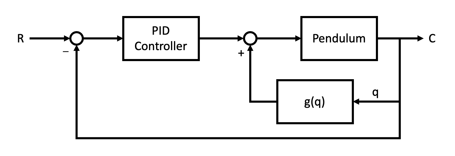
The gravity compensation method involves extracting the \(g(q)\) term from the equation of motion and incorporating it into the feedback loop of the PID controller. This approach allows the control system to proactively counteract gravitational effects, leading to more precise and efficient control. Figure 1 illustrates the block diagram of this enhanced control system.

1. Principles of PID Control with Gravity Compensation

The PID control with gravity compensation method combines the simplicity of PID control with the advantages of model-based control. The key principles are:

1. Traditional PID control for error correction
2. Gravity compensation to counteract the effects of gravity on the system
3. Integration of these components to create a more robust control system

The control law can be expressed as:

\[\tau = K_p e + K_i \int e dt + K_d \dot{e} + g(q) \tag{2}\]

Where \(K_p\), \(K_i\), and \(K_d\) are the proportional, integral, and derivative gains respectively, \(e\) is the error, and \(g(q)\) is the gravity compensation term.

2. Advantages and Limitations

Advantages:

• Improved stability and performance compared to standard PID control
• Reduced settling time and overshoot
• Better handling of gravitational nonlinearities
• Relatively simple implementation compared to full nonlinear control methods

Limitations:

• Still does not account for all nonlinear dynamics (e.g., Coriolis and centrifugal forces)
• Requires accurate modeling of the gravitational effects
• May not be as effective for highly dynamic or rapidly changing systems

3. Applications

This combined PID and gravity compensation approach finds applications in various fields:

1. Robotic manipulators: Improving positioning accuracy in industrial robots
2. Aerospace: Attitude control of spacecraft and satellites
3. Mechanical systems: Control of cranes and gantry systems
4. Biomechanics: Design of prosthetic limbs and exoskeletons
5. Manufacturing: Precision control in CNC machines and 3D printers

In the following sections, we will delve deeper into the implementation and advantages of this combined PID and gravity compensation approach, demonstrating its effectiveness in controlling triple-link mechanisms.

II. A Multi-Link Mechanism with a Fixed Base

A. Overall System

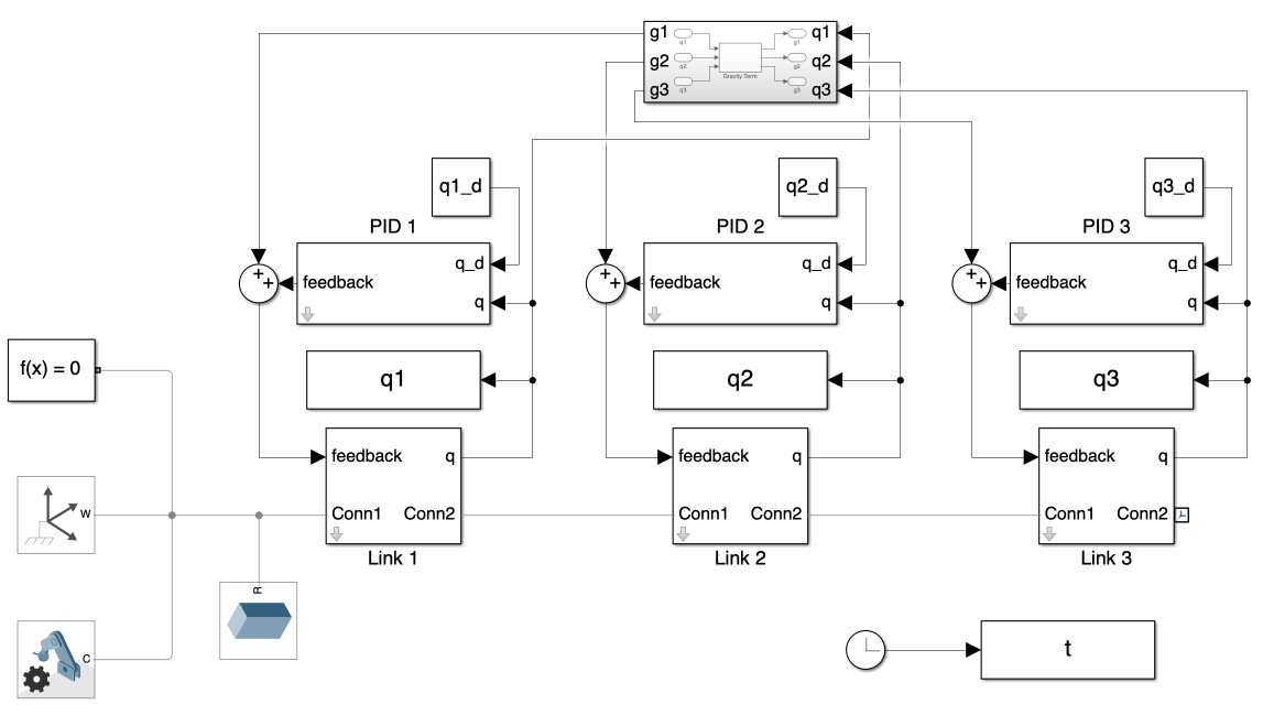
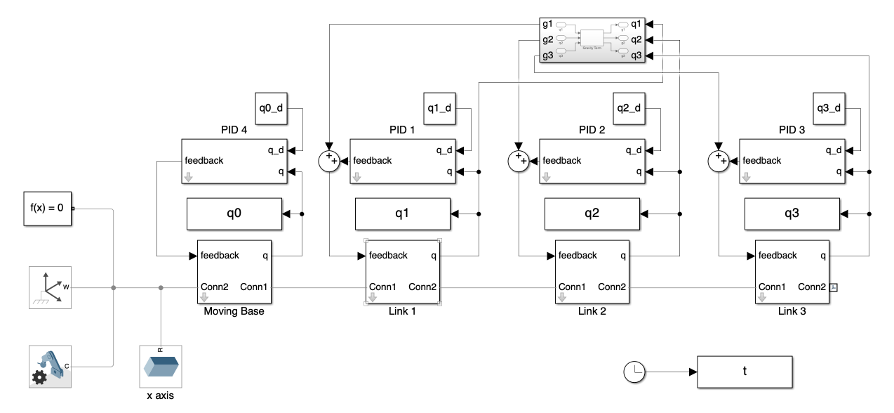
The overall system is depicted in Figure 1. This system closely resembles that of Day 2, with the addition of a gravity calculation block. The angular displacement of each joint is fed into both the PID controller block and the gravity calculation block. Each block calculates its own feedback, which is then combined to determine the feedback torque needed to actuate the joints.

B. Gravity Calculation Block

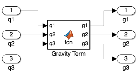
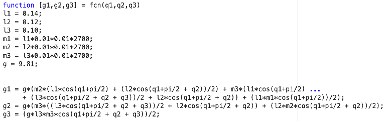
The gravity calculation block is relatively straightforward. Calculating the gravity term through circuit design is complex and time-consuming. Instead, we use a “MATLAB Function block,” as illustrated in Figure 2. This block allows us to write a MATLAB script to compute the gravity term, which is detailed in Figure 3.

Extracting the gravity term from the equation of motion is straightforward. Given the symbolic representation of the motion equation, we apply partial differentiation with respect to \(g\), the gravitational constant, to isolate the gravity-related terms. After this differentiation, we multiply the result by \(g\) again to reintegrate the gravity constant into the equation. Additionally, we replace \(q_1\) with \(q_1 + \frac{\pi}{2}\) in the equation, as we used \(\theta\) as the variable instead of \(q\), in Day 3.

C. Simulation

In this section, we explore the simulation, focusing on both tracking and regulation capabilities of the system with fixed base. Through these simulations, we aim to validate the effectiveness of the controllers in maintaining trajectory accuracy (tracking) and stabilizing the system against disturbances (regulation).

1) Tracking

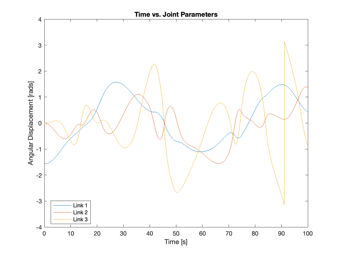
Firstly, we set all the gains of the PID controller to zero to test if compensating gravity alone could track the reference input. The results demonstrated that it could neither track the reference input nor stabilize the system. We ran the simulation for up to 10,000 seconds, but the system remained unstable. It resembled an upside-down, slow-moving triple-link mechanism, which also exhibited chaotic behavior. The simulation video and the graph for each joint parameter are displayed in Video 1 and Figure 5, respectively.

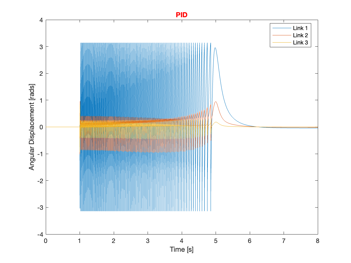
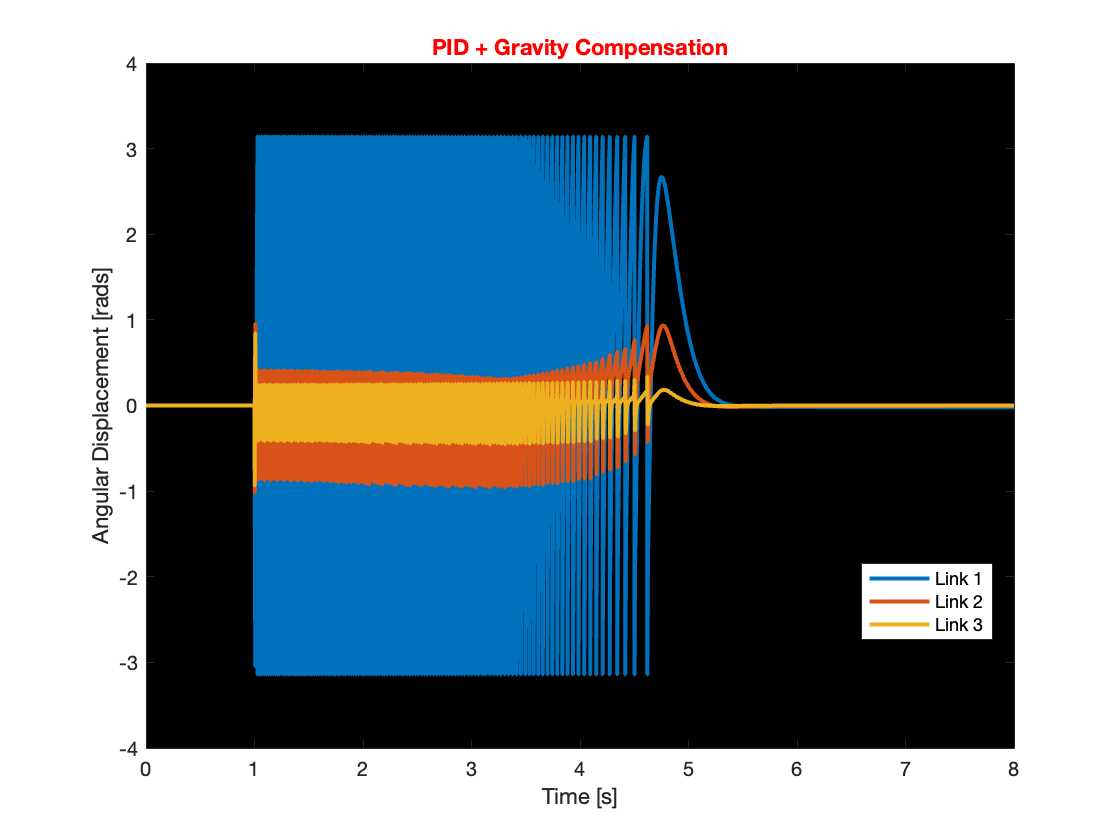
Following the initial simulation, we executed a second simulation using the same PID controller settings as on Day 2, incorporating the gravity calculation block as well. This simulation was intended to assess the impact of gravity compensation on the system’s overall performance. The results, as depicted in Video 2 and Figure 6, indicate that gravity compensation slightly enhanced the tracking speed. In Video 2, the left multi-link mechanism is controlled solely by a PID controller, while the right multi-link mechanism utilizes both PID control and gravity compensation. In Figure 6, you can slide the graphs to switch between the PID (left) and PID + gravity compensation (right) data for comparison.

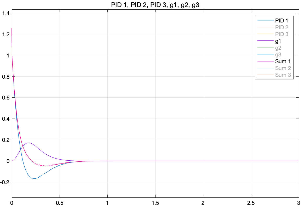
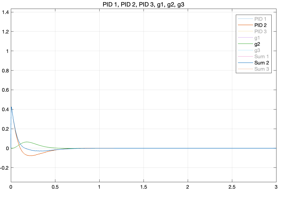
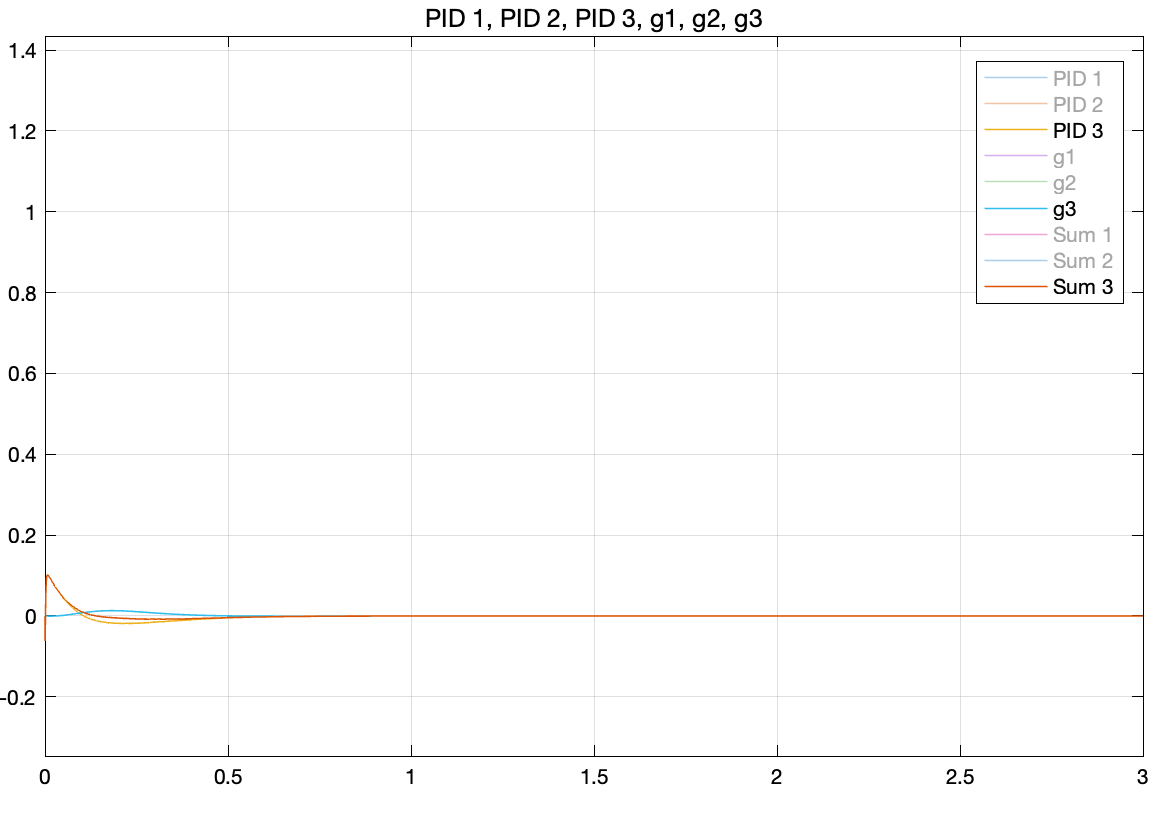
Lastly, we extracted the feedback data from each PID controller and the gravity calculation block to analyze how the gravity term influences the overall feedback. Figures 7 through 9 display the feedback from each joint.

To reduce the torque overshoot, the PID controller’s gain can be adjusted by decreasing \(K_p\) or increasing \(K_d\), though this tends to slow the system. However, as demonstrated in Figures 7 through 9, the feedback from gravity compensation acts to counterbalance the PID controller, effectively reducing torque overshoot without significantly affecting the system’s transient response time. This allows for quicker convergence.

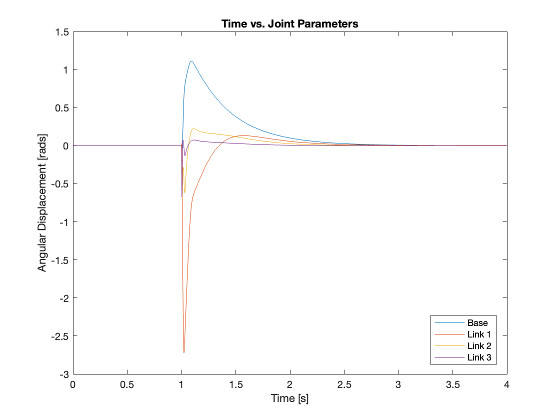
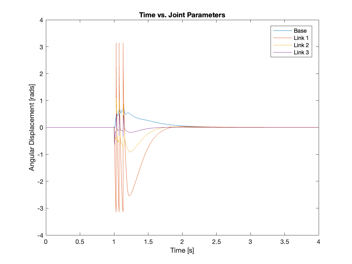
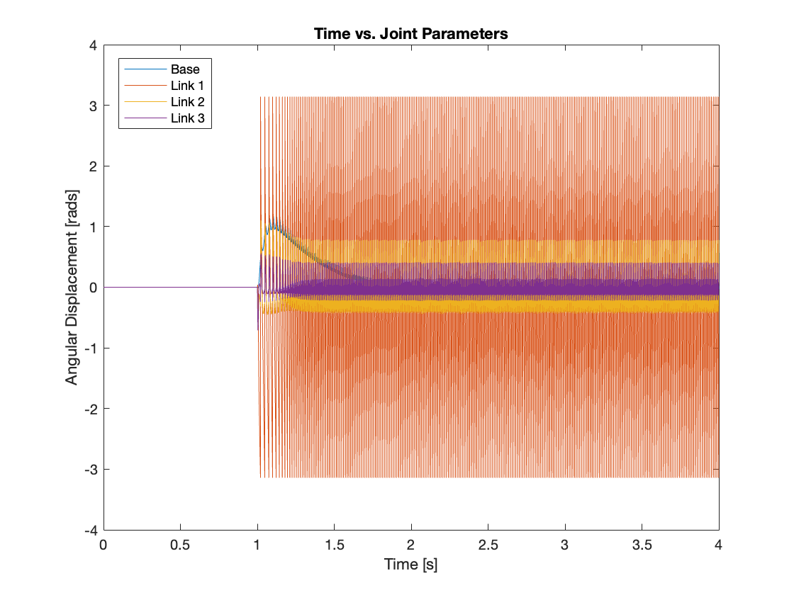
2) Regulation

Through simulation of the tracking, it was found that compensating for gravity aids in faster system convergence and reduces overshoot. Additionally, systems with gravity compensation restabilized more quickly and exhibited smaller overshoots compared to those without it under similar conditions when dealing with small disturbances. However, for larger disturbances, does gravity compensation resolve issues such as overreaction and destabilization? The answer is no. Despite implementing gravity compensation, these issues remained unresolved for larger disturbances. This conclusion is supported by the results shown in Videos 3 through 5 and Figures 10 through 12.

---

---

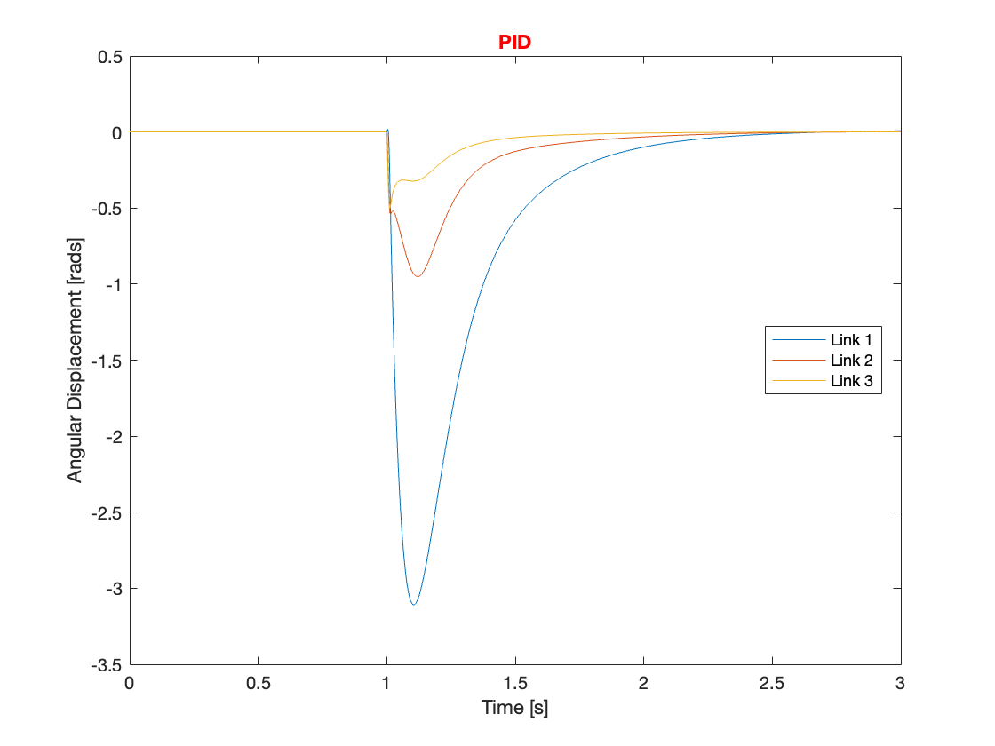
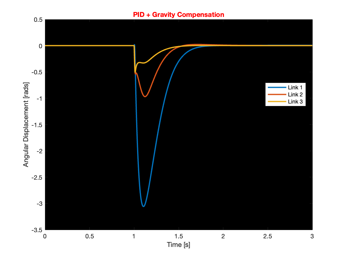
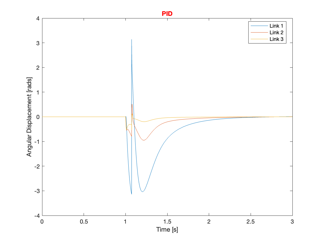
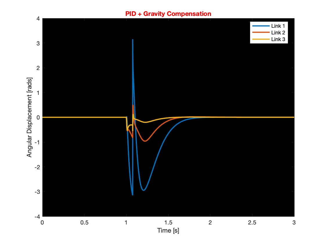
Even though gravity compensation could not resolve the overreaction issue, it was observed that systems with gravity compensation recovered more quickly than those without. This quicker recovery was achieved by maintaining a faster angular speed when the angular displacement was small. Through simulation, it was determined that gravity compensation is more effective when there is a small angular displacement. Consequently, under conditions of small angular displacement, using a PID controller with gravity compensation can efficiently manage the system, optimizing performance and stability.

III. A Multi-Link Mechanism with a Moving Base

A. Overall System

Thankfully, the base moves only along the x-axis, and there are no gravity terms related to the base. As a result, this setup closely resembles a system with a fixed base. The overall system configuration is depicted in Figure 13.

B. Simulation

Since there were no significant changes, and we’ve already discussed all the findings in the fixed base section, we will present the results using the same parameters as Day 2. The results demonstrate faster stabilization.

1) Tracking

Videos 6 through 9 and Figures 14 through 17 demonstrate the tracking capabilities of the controller across various initial states in the simulation of a triple-link mechanism with a moving base. The initial states are defined as follows: for \(q_1\), the values are (180, -90, 150, 190); for \(q_2\), the values are (0, 0, 180, 180); and for \(q_3\), the values are (0, 0, 180, -110).

2) Regulation

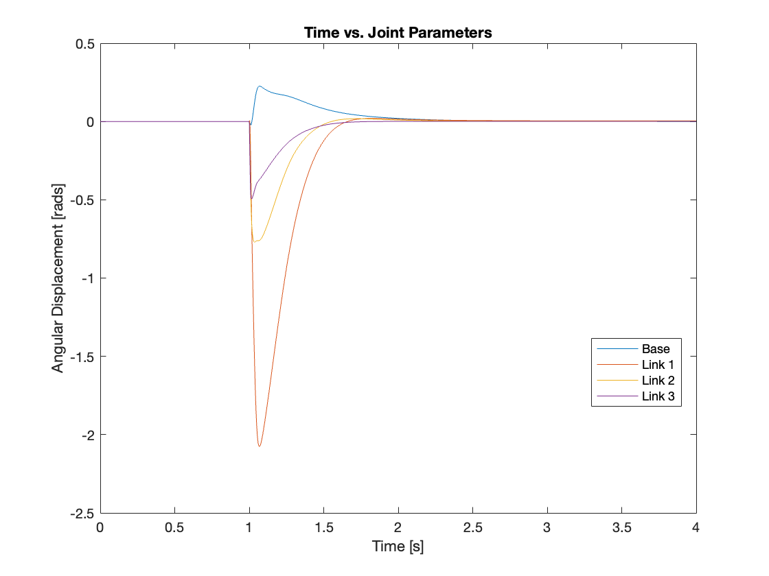
Videos 10 through 13 and Figures 18 through 21 demonstrate the tracking capabilities of the controller across various initial states in the simulation of a triple-link mechanism with a moving base. All the initial states, \(q\), were set to 0. Adjustments were then made to the density of the base and the magnitude of disturbance. The densities, denoted as \(\rho_0\), are set to \((2700, 2700, 50000, 50000) kg/m^3\), and the forces, denoted as \(f\), are \((100, 500, 300, 500) N\).

IV. Conclusion and Moving Forward

Today, we managed a fully actuated multi-link mechanism using a PID controller complemented by gravity compensation. The simulations revealed that gravity compensation significantly enhances stabilization by maintaining a high angular velocity when the angular displacement is minimal. Upon examining the torque feedback, we observed that gravity compensation acts as a counterbalance to the feedback from the PID, effectively reducing torque overshoot. Therefore, in scenarios involving only slight angular displacements, incorporating gravity compensation can markedly improve system performance.

During today’s simulations, we realized that simulating the fixed base system might be time-consuming. Hence, starting from Day 5, we will omit simulations of the fixed base system. Stay tuned for more updates as we continue exploring the fascinating realm of multi-link mechanisms and tackle the challenges associated with controlling chaotic systems!

You can find the Simulink model on my GitHub repository.