This post builds upon the lecture by Dr. Jun Ueda, exploring an enhanced control system for multi-link mechanisms.

I. Introduction

On Day 4, we realized that while a PID controller with gravity compensation stabilizes the system faster, it often struggles with overreactions and potential destabilizations. This occurs because it focuses solely on angular positions, neglecting angular velocities.

Building on the equations of motion derived on Day 3 for the triple-link mechanism:

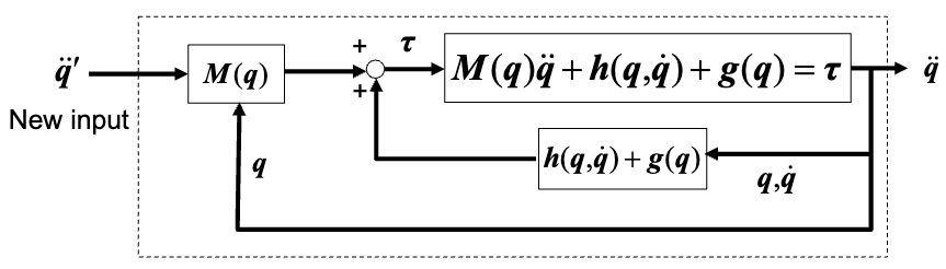
\[\tau = M(q)\ddot{q} + h(q, \dot{q}) + g(q) \tag{1}\]

Where:

• M(q) (Inertial Matrix): Represents the system’s inertial properties, describing how the mechanism resists acceleration in response to applied torques.
• h(q, ̇q) (Coriolis and Centrifugal Terms): Accounts for the Coriolis and centrifugal forces, which depend on the system’s velocities and rotational dynamics.
• g(q) (Gravitational Term): Describes the torques induced by gravitational forces acting on each component of the mechanism.

Today, we introduce a nonlinear control system that combines a PID controller with the computed torque method. This system tackles the nonlinear dynamics effectively, compensating for gravity and dynamic forces while integrating displacement and velocity feedback.

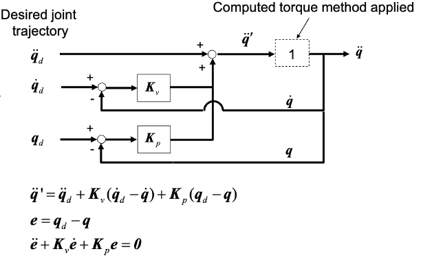
The revised block diagrams in Figures 1 and 2 illustrate how the computed torque method enhances the PID controller by leveraging the system’s full dynamics to accurately predict and correct disturbances. These diagrams are referenced from Dr. Jun Ueda’s lecture slides.

1. Principles of Computed Torque Method

The computed torque method is a feedback linearization technique that aims to cancel out the nonlinear dynamics of the system. It works by:

1. Using the system’s dynamic model to compute the required torques.
2. Applying these torques to counteract the nonlinear terms in the system’s dynamics.
3. Resulting in a linearized system that can be controlled using linear control techniques.

The method is based on the inverse dynamics of the system, where the control input is calculated as:

\[\tau = M(q)\ddot{q}' + h(q, \dot{q}) + g(q)\]

Here, \(\ddot{q}'\) is the new input that includes the desired acceleration and error feedback terms.

2. Advantages and Limitations

Advantages:

• Effective handling of nonlinear dynamics
• Improved tracking accuracy and stability
• Reduced need for extensive parameter tuning
• Enhanced performance in complex, multi-DOF systems

Limitations:

• Requires accurate system model for optimal performance
• Computationally intensive, especially for complex systems
• Sensitivity to modeling errors and parameter uncertainties
• Potential for instability if model inaccuracies are significant

3. Applications

The computed torque method finds applications in various fields requiring precise control of nonlinear systems:

1. Robotics: Industrial manipulators, humanoid robots
2. Aerospace: Aircraft and spacecraft control systems
3. Automotive: Advanced suspension systems, autonomous vehicles
4. Manufacturing: CNC machines, precision assembly
5. Biomechanics: Prosthetic limbs, exoskeletons
6. Process control: Chemical reactors, distillation columns

II. Mathematical Modeling and Analysis

1. Linearized Dynamics

The linearized system dynamics are introduced using the equation:

\[\tau = M(q)\ddot{q}' + h(q, \dot{q}) + g(q)\]

This formula for $\tau$, based on the computed input $\ddot{q}’$, quantifies the total force required to achieve the control objectives. The dynamics without control input adjustment, given by Equation 1, are aligned with this formulation to yield:

\[M(q)\ddot{q}' + h(q, \dot{q}) + g(q) = M(q)\ddot{q} + h(q, \dot{q}) + g(q) \Rightarrow \ddot{q}' = \ddot{q} \tag{2}\]

This result indicates that under ideal control conditions, where the system accurately follows the control input, $\ddot{q}’$ aligns with the actual acceleration $\ddot{q}$ needed to match the desired trajectory.

2. Input Through PID Controller

The new input $\ddot{q}’$ is formulated using a PID controller to correct the error, described by the equation:

\[\ddot{q}' = \ddot{q}_d + K_d(\dot{q}_d - \dot{q}) + K_p(q_d - q) + K_i\int{(q_d - q)}dt \tag{3}\]

Using Equations 2 and 3, the dynamics correction can be expressed as:

\[(\ddot{q}_d - \ddot{q}) + K_d(\dot{q}_d - \dot{q}) + K_p(q_d - q) + K_i\int{(q_d - q)}dt \tag{4}\]

3. Define the Error Dynamics

The tracking error is foundational for deriving the system’s dynamics, defined by:

\[e = q_d - q \tag{5}\]

This definition facilitates the expression of derivatives in terms of error:

\[\dot{e} = \dot{q}_ d - \dot{q}, \quad \ddot{e} = \ddot{q}_d - \ddot{q} \tag{6}\]

4. Error Dynamics Equation

Derived from Equation 4 by substituting Equations 5 and 6, the full error dynamics is given by:

\[\ddot{e} + K_d\dot{e} + K_pe + K_i \int{e}dt = 0 \tag{7}\]

This equation establishes the control dynamics under the implemented inputs, serving as a crucial indicator for system stability.

5. Stability Analysis

The stability of the system is evaluated using the Routh–Hurwitz criterion. According to this criterion, the system is considered stable if:

\[K_dK_p > K_i \tag{8}\]

This inequality must hold to ensure that the system approaches stability, meaning that as time approaches infinity, the error effectively reduces to zero:

\[t \rightarrow \infty \Rightarrow e \rightarrow 0 \tag{9}\]

III. Simulink Implementation

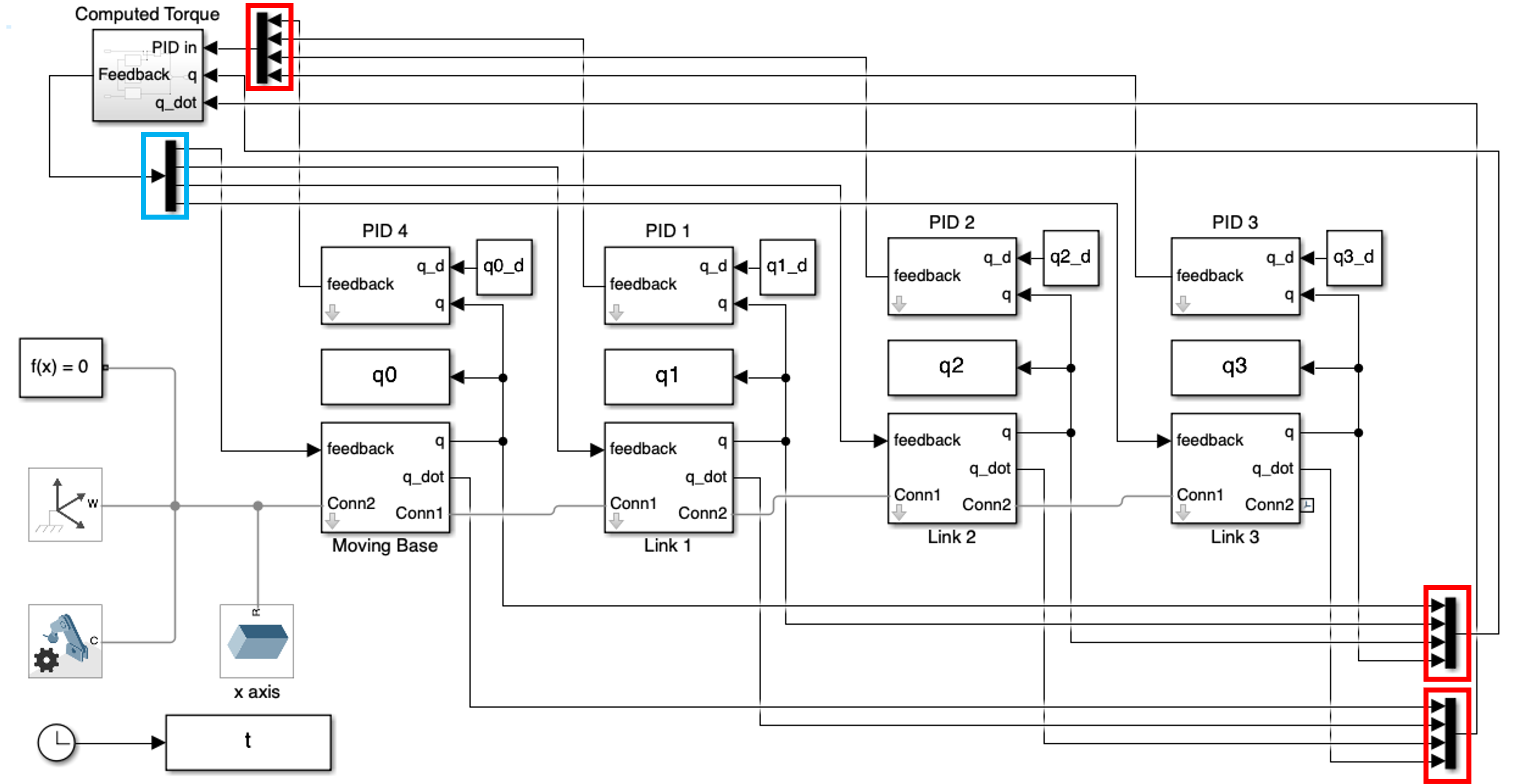
1. Overall System

The overall system is illustrated in Figure 3. As observed, the system architecture bears resemblance to a traditional PID control setup but incorporates additional subsystems and components to enhance functionality. These new elements are the “MUX (Red box)” and “DEMUX (Blue box)”, which play critical roles in handling signal matrices within the control loop.

• MUX (Red box): The Multiplexer (MUX) is used to combine multiple single signals into a single matrix. This is particularly useful in control systems like ours where multiple input signals need to be processed simultaneously in a compact form. In Simulink, a MUX block simplifies system connections by aggregating several input lines into one output, feeding into systems that require a single input stream containing multiple signals.

• DEMUX (Blue box): Conversely, the Demultiplexer (DEMUX) is used to split a matrix into its component single signals. This is essential for systems that process signals in a matrix form but then require individual signal handling downstream. In Simulink, the DEMUX block facilitates the distribution of a single input containing multiple data points into multiple outputs, which can then be directed to specific parts of the system.

By channeling matrices through a “Computed Torque” subsystem using these blocks, the system is able to compute and output a new feedback torque that is more accurately aligned with the dynamic requirements of the controlled process.

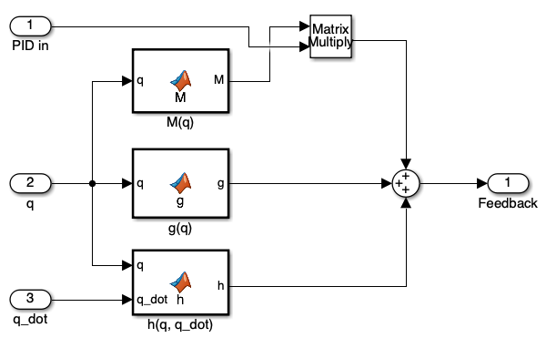
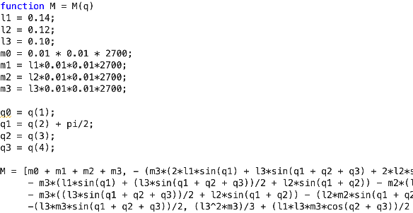
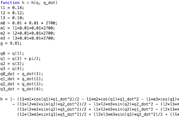
2. Computed Torque Method Block

Calculating torque through circuit design can be complex and time-consuming. Similar to the gravity calculation block described on Day 4, the computed torque method block simplifies this process. As depicted in Figure 4 and detailed through MATLAB scripts in Figures 5-7, we utilize “MATLAB Function blocks” within the computed torque block. These blocks allow us to script MATLAB code directly to compute each term of Equation 1. It’s important to note that we used a Matrix multiplication block instead of an element-wise multiplication block because Equation 1 involves matrix calculations, necessitating proper alignment and dimension matching of matrices.

• \(M(q)\): This block computes the mass matrix (M) from Equation 1, which is critical as it reflects the system’s inertia. The matrix \(M\) is derived by partially differentiating Equation 1 with respect to each angular acceleration.

• \(h(q, \dot{q})\): This block calculates the Coriolis and centrifugal forces, represented as the second term in Equation 1. These dynamic forces are crucial for accurately modeling the behavior of rotating systems. The matrix \(h\) is obtained by isolating these forces in Equation 1, which can be done by subtracting \(M(q)\ddot{q} + g(q)\) from the total torque \(\tau\).

• \(g(q)\): This block computes the gravitational forces, consistent with the gravity block used on Day 4. This ensures that gravitational effects are accurately integrated into the torque computation. The matrix \(g\) is derived by isolating the gravitational term in Equation 1, which involves differentiating the gravitational components and then reintegrating them into the model.

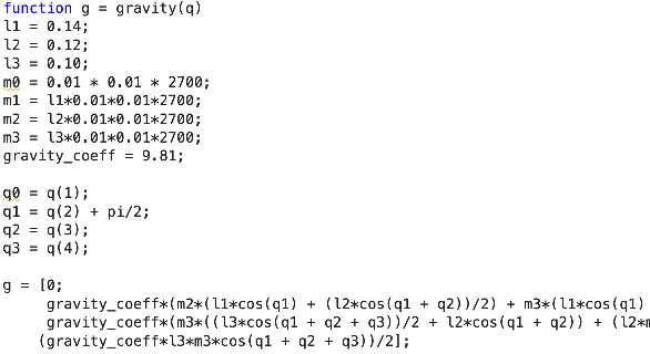
It’s important to note that \(q1\) has been defined as \(q(2) + \frac{\pi}{2}\). This definition is used because \(\theta_1\) is set as \(\theta_1 = \frac{\pi}{2} + q_1\) on Day 3.

III. Simulation

In this section, we explore the simulation, focusing on both tracking and regulation capabilities of the multi-link mechanism control system. Through these simulations, we aim to validate the effectiveness of the controllers in maintaining trajectory accuracy (tracking) and stabilizing the system against disturbances (regulation).

1. Tracking

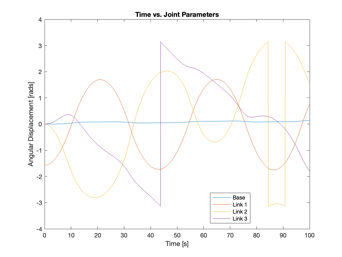
a) No PID Input

Initially, we set all the gains of the PID controller to zero to evaluate whether the computed torque block alone could effectively track the reference input. The results indicated that without the PID gains, the system failed to track the reference input and could not stabilize. We extended the simulation to 10,000 seconds, but the system remained unstable throughout, exhibiting behavior akin to an upside-down, slowly oscillating triple-link mechanism, which also showed signs of chaotic dynamics. This instability likely stems from the absence of error correction typically provided by the PID controller. The simulation video and the graph depicting each joint’s parameters are presented in Video 1 and Figure 8, respectively.

b) Varying PID gains

1) \(K_p = 0.1, K_i = 0.001, K_d = 0.01\)

we began with very small PID controller gains, anticipating that the results would be similar to those without PID input. However, the outcome was entirely different from what we had expected. The system rotated counterclockwise and was not fully chaotic. While Base 1, Link 1, and Link 3 became marginally stable, Link 2 remained unstable. Video 2 and Figure 9 depict the initial phase of the triple-link mechanism, while Video 3 and Figure 10 showcase the middle phase.

2) \(K_p = 1, K_i = 0.01, K_d = 0.1\)

When we increased the gains slightly, the multi-link mechanism stabilized after oscillating for an extended period. An interesting observation was the lag in oscillation between the links. The maximum amplitude of Link 1 occurs first, followed by Link 2, and then Link 3. Also, intriguingly, when all the links are oscillating, the motion resembles that of a tail. Video 4 and Figure 11 display the results of the simulation.

3) \(K_p = 100, K_i = 1, K_d = 20\)

we further increased the gain, resulting in rapid stabilization of the multi-link mechanism. An interesting behavior observed was that the multi-link mechanism maintained an almost straight posture during its movement. Video 5 and Figure 12 display the results of the simulation.

4) \(K_p = 10^6, K_i = 10^4, K_d = 2\times10^5\)

An interesting discovery was that although we could increase the PID gains indefinitely, the system’s performance has a distinct upper limit. Despite higher PID gains, performance actually deteriorated. It appears that for this controller, iterative testing is necessary to determine the optimal set of gains. Video 6 and Figure 12 compare the PID settings of \((K_p, K_i, K_d) = (100, 1, 20) and (10^6, 10^4, 2 \times 10^5)\).

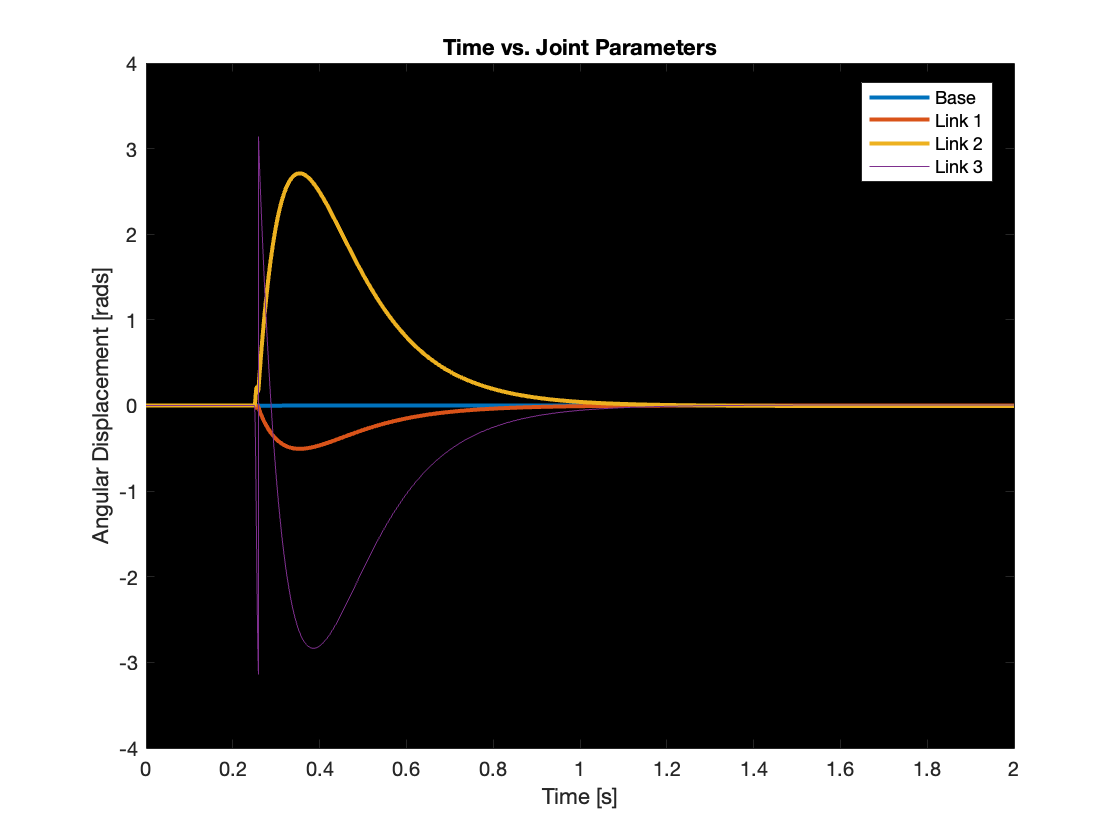
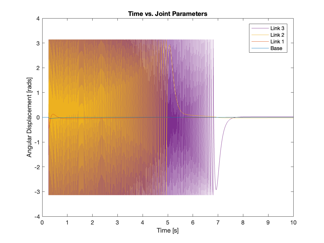
5) \(K_p = 10, K_i = 300, K_d = 20\) (Unstable System)

In the final phase of our tracking experiment, we simulated an unstable system characterized by the condition \(K_dK_p < K_i\). As demonstrated in Video 7, Link 1, which experienced the most significant initial perturbation, exhibited signs of instability first. This instability progressively influenced Link 2 and Link 3, causing their perturbations to intensify. Ultimately, all links displayed unstable behavior. Figure 14 vividly illustrates this phenomenon, showing the angular positions of Link 2 and Link 3 diverging over time.

2. Regulation

For the controller regulation simulation, we configured the initial joint PID gains to (100, 1, 20), which yielded the best performance in the tracking simulation. Additionally, we set the PID gains for the moving base to (10, 0.01, 4).

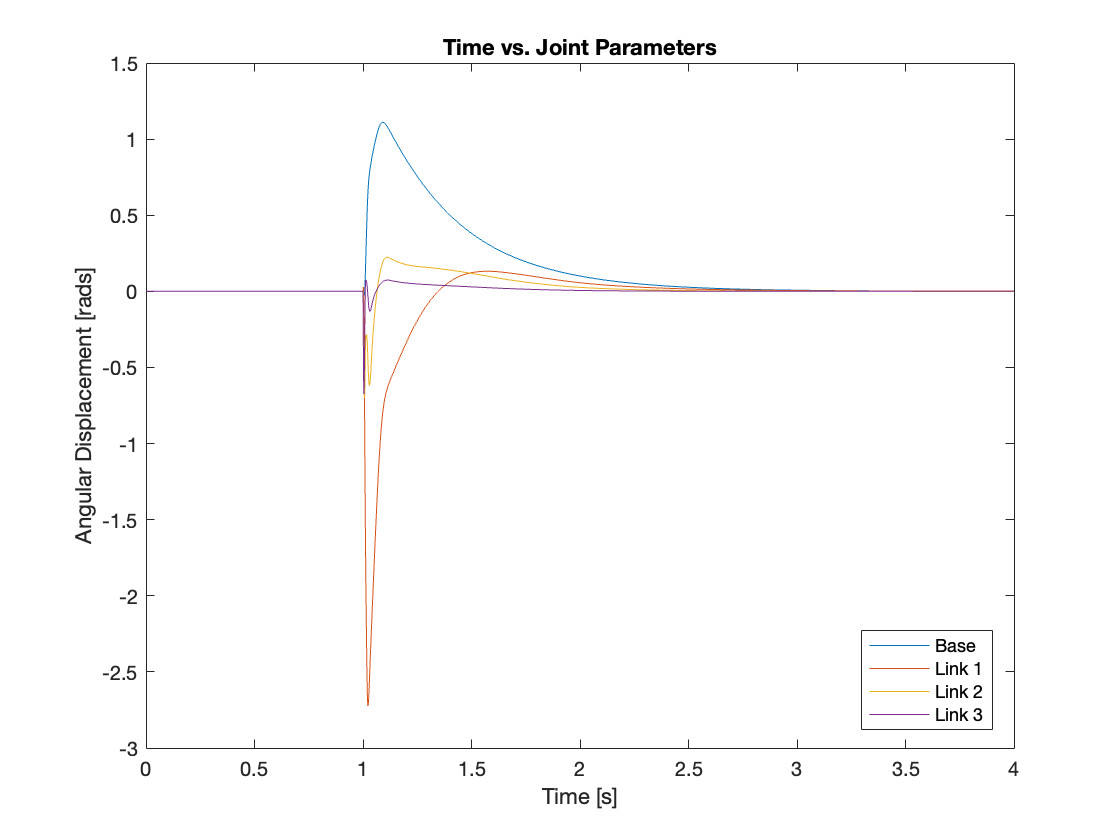
1) \(\rho_0 = 2700kg/m^3, F = 100N\)

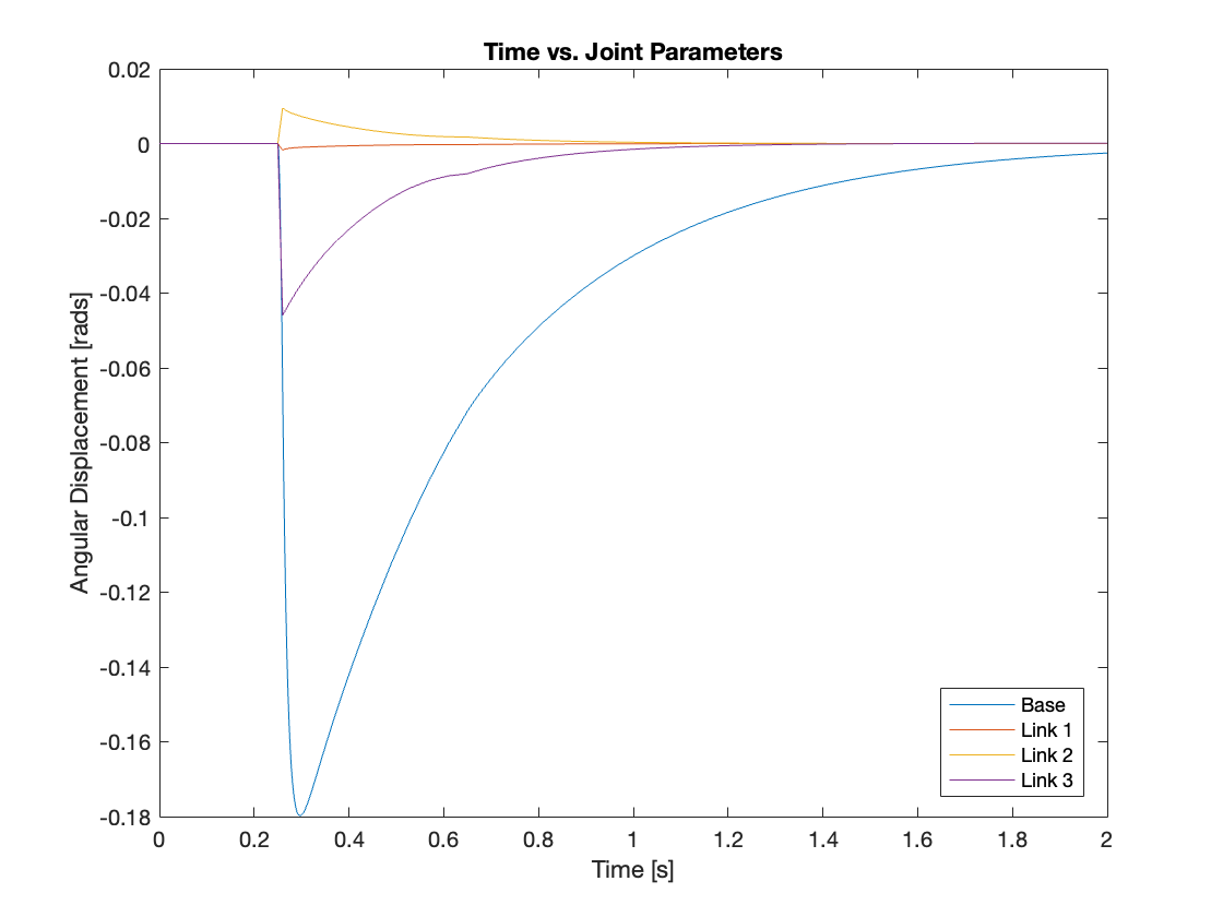
Compared to the PID + gravity compensation controller, there was less force propagation through the links, with most of the force being compensated by the rotation of Link 3, and the base remaining almost stationary. Video 7 and Figure 14 compare the simulations of PID + Gravity Compensation (PID + g) and PID + Computed Torque (PID + t).

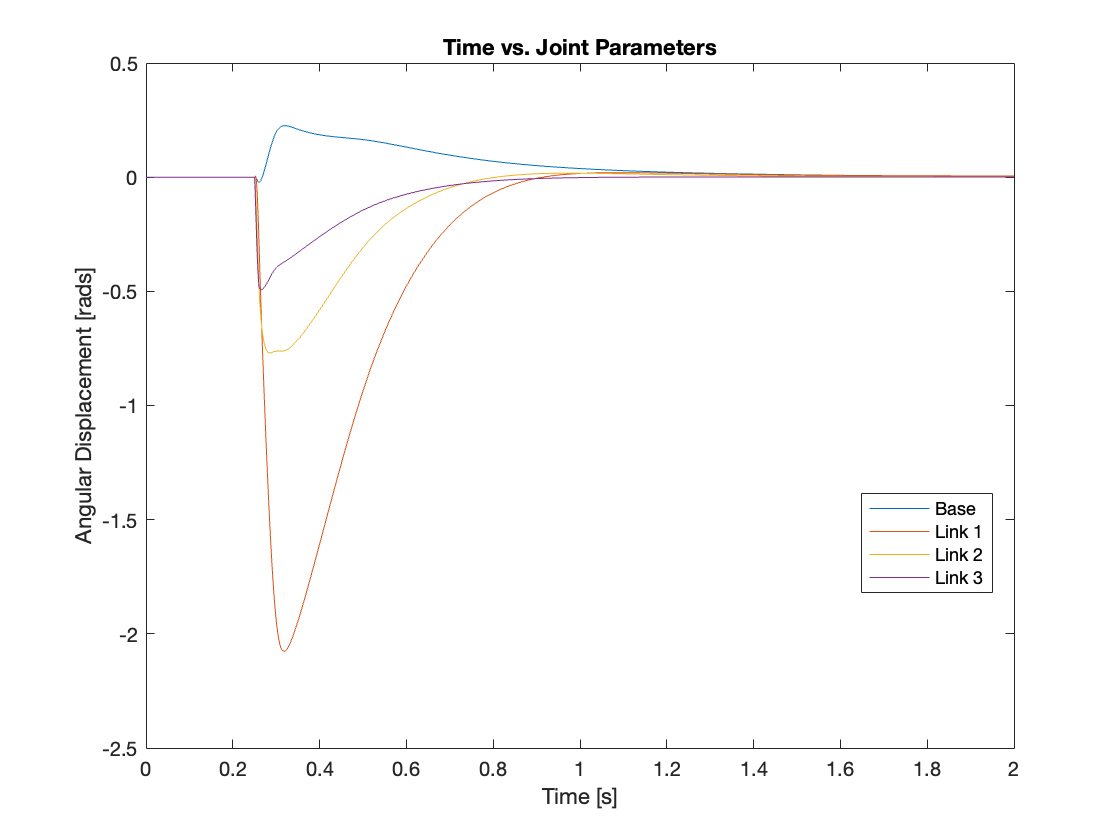
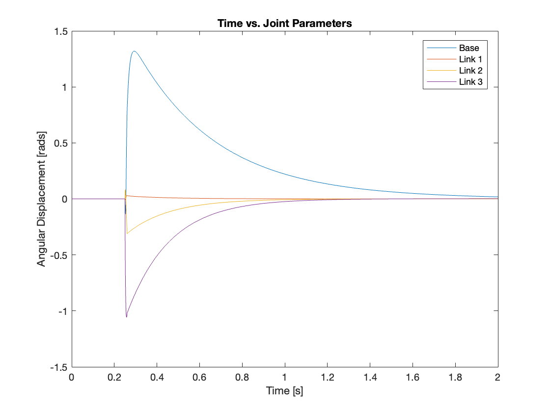
2) \(\rho_0 = 2700kg/m^3, F = 500N\)

In Video 8, the “PID + gravity compensation” method enabled force to propagate through the links, requiring all the actuators at the joints to exert a similar effort to stabilize the system. In contrast, Video 9 demonstrates the “PID + computed torque” method, where force propagation was significantly reduced, concentrating the effort predominantly on Joint 3. This led to a longer stabilization time for the system, as the impact was not effectively absorbed by all the links and the base, but was largely managed by link 3. The differences in actuator displacement, as shown in Figure 15 and Figure 16, related to the difference in the distribution of impact absorption between the two methods.

3) \(\rho_0 = 2700kg/m^3, F = 500N, K_p = 10^6, K_i = 10^4, K_d = 2\times10^5\)

As observed during the tracking simulation, we was able to set the PID gains extremely high. With these settings, the regulation was effectively managed; the links hardly moved. Interestingly, the base moved toward the left, opposite to the direction of the external force. This is due to the efforts of the joints. The results are showcased in Video 10 and Figure 17.

3) \(\rho_0 = 2700kg/m^3, F = 50000N, K_p = 10^6, K_i = 10^4, K_d = 2\times10^5\)

However, as demonstrated in Video 11 and Figure 18, if the force is sufficiently strong, the base moves to the right, aligning with the direction of the external force.

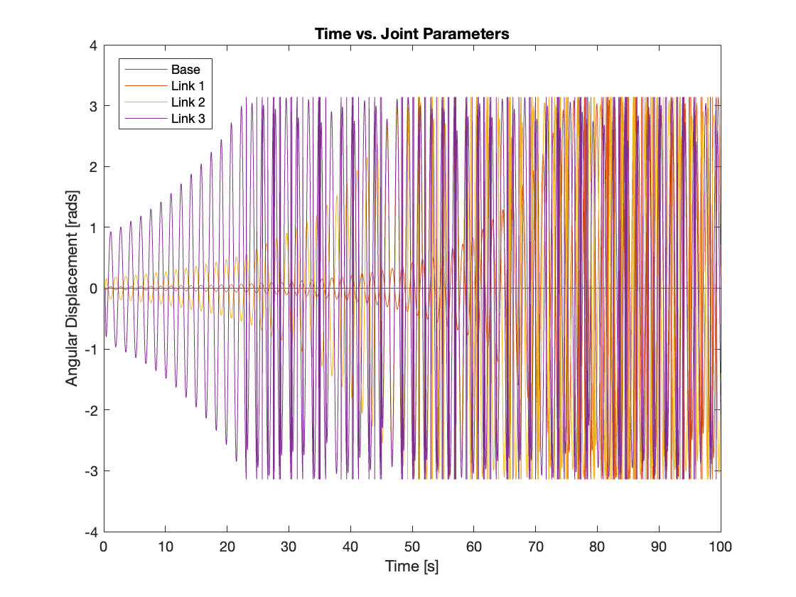
4) \(\rho_0 = 2700kg/m^3, F = 1N, K_p = 10, K_i = 300, K_d = 20 (Unstable System)\)

Similar to the tracking simulation, we also simulated the regulation of an unstable system, defined by the condition \(K_dK_p < K_i\). In this configuration, even a minor perturbation can cause the system to diverge rapidly. This sensitivity to disturbances highlights the challenges of controlling such a system. In Video 12 and Figure 20, you can observe how these tiny perturbations escalated, leading to increasingly significant deviations from the stable state.

IV. Conclusion

Today, we enhanced the control of a fully actuated multi-link mechanism using a PID controller integrated with the computed torque method. Compared to standalone PID control and PID with gravity compensation, this approach demonstrated superior performance. One notable advantage is that this system achieves full linearity through feedback linearization, simplifying the control loop.

During the simulation, we observed two key findings: First, while the gains of the PID controller can be increased significantly, this does not necessarily translate to improved performance. Second, although the computed torque method markedly enhances system performance, it does not address inherent PID limitations such as the potential for overreaction. This suggests that while the PID controller remains a component, some of its fundamental drawbacks persist.

Through Days 4 and 5, we studied and implemented the feedback linearization method for nonlinear systems. Now, equipped with this understanding, we am eager to explore a variety of other nonlinear control strategies. Stay tuned for more updates as we continue to explore the fascinating world of multi-link mechanisms and tackle the challenges associated with controlling chaotic systems!

You can find the Simulink model on my GitHub repository.