Before diving into the technicalities, we must address a fundamental challenge encountered while implementing nonlinear controllers for multi-link mechanisms: the inherent high nonlinearity of these systems. This complexity can significantly complicate the design and effectiveness of controllers, posing a substantial barrier to achieving desired performance and stability.

Given these challenges, and with the goal of this post to introduce and explore various controller designs, we have decided to simplify the scenario slightly by reducing the number of links in our mechanisms. This approach will help in isolating and understanding the specific impacts and benefits of each control strategy without the overwhelming interactions of a highly complex system.

I. Introduction

State Feedback Control is a fundamental technique in modern control theory that forms the basis for many advanced control strategies, including the Linear Quadratic Regulator (LQR). This approach allows for precise manipulation of a system’s behavior by feeding back information about its current state. In this post, we’ll explore the principles, mathematics, advantages, limitations, and applications of State Feedback Control.

1. Principles of State Feedback Control

a) System Model

State Feedback Control is designed for systems that can be described by a state-space model:

Where:

• \(x\) is the state vector
• \(u\) is the control input vector
• \(y\) is the output vector
• \(A\), \(B\), \(C\), and \(D\) are matrices defining the system dynamics

b) Control Law

The core idea of State Feedback Control is to make the control input a linear function of the state:

Here, \(K\) is the feedback gain matrix that is designed to achieve desired system behavior.

c) Advantages of State Feedback Control

State Feedback Control offers several key advantages:

• Flexibility: It allows for precise control over individual state variables, enabling fine-tuning of system response.
• Stability: Proper design of the gain matrix K can stabilize inherently unstable systems.
• Optimality: When combined with optimal control techniques (like LQR), it can minimize control effort while achieving desired performance.
• Robustness: It can provide a degree of robustness to certain types of disturbances and model uncertainties.

d) Limitations of State Feedback Control

Despite its strengths, State Feedback Control has some limitations:

• State Measurement: It requires accurate measurement or estimation of all state variables, which can be challenging in some systems.
• Model Dependence: The effectiveness of the control law depends on the accuracy of the system model.
• Linear Systems: Basic State Feedback Control is designed for linear systems; nonlinear systems require more advanced techniques.
• Gain Selection: Choosing appropriate gains can be complex, especially for systems with many states.

e) Applications of State Feedback Control

State Feedback Control finds wide application across various fields:

1. Aerospace: Aircraft flight control systems, satellite attitude control
2. Robotics: Robot arm positioning, balance control in humanoid robots
3. Automotive: Active suspension systems, electronic stability control
4. Process Control: Temperature and pressure regulation in chemical processes
5. Power Systems: Voltage and frequency control in electrical grids
6. Mechatronics: Precision positioning in manufacturing equipment

2. Principles of Pole Placement Method

a) Pole Placement Method

The pole placement method is a powerful technique for designing the feedback gain matrix \(K\) in state feedback control. This method allows us to directly specify the desired eigenvalues of the closed-loop system, which in turn determines its dynamic response characteristics.

Here’s how it works:

1. Closed-loop System: When we apply the state feedback control law \(u = -Kx\) to our system \(\dot{x} = Ax + Bu\), we get the closed-loop system:

   \[\dot{x} = (A - BK)x \tag{4}\]

2. Eigenvalues: The eigenvalues of \((A - BK)\) determine the system’s stability and transient response. These are the roots of the characteristic equation:

   \[det(sI - (A - BK)) = 0 \tag{5}\]

3. Desired Poles: we choose a set of desired eigenvalues \(\{\lambda_1, \lambda_2, ..., \lambda_n\}\) based on our performance requirements (stability, settling time, overshoot, etc.).

4. Characteristic Polynomial: we form the desired characteristic polynomial:

   \[\alpha(s) = (s - \lambda_1)(s - \lambda_2)...(s - \lambda_n) \tag{6}\]

5. Solving for K: we then solve for \(K\) by equating the coefficients of \(\alpha(s)\) with those of \(det(sI - (A - BK))\).

For example, in a second-order system, if we want the closed-loop poles at \(s = -2 \pm j2\), our desired characteristic polynomial would be:

we would then solve for \(K\) to make \(det(sI - (A - BK))\) equal to this polynomial.

The pole placement method gives us direct control over the system’s eigenvalues, allowing us to shape its response precisely. However, it requires that the system be completely state controllable.

b) Advantages of Pole Placement

• Direct Control: Allows precise specification of system dynamics.
• Intuitive Design: Engineers can relate pole locations to time-domain performance.
• Flexibility: Can achieve various performance objectives by appropriate pole selection.

c) Limitations of Pole Placement

• Controllability Requirement: The system must be completely state controllable.
• Sensitivity: The resulting system can be sensitive to model uncertainties.
• Complexity: For high-order systems, selecting appropriate poles can be challenging.
• Control Effort: May result in high control efforts if poles are placed too far left in the s-plane.

3. Principles of Controllability

Controllability is a fundamental concept in control theory that plays a crucial role in the design and analysis of control systems, particularly in state feedback control and pole placement methods.

a) Definition of Controllability

A system is said to be controllable if it’s possible to transfer the system from any initial state to any desired final state within a finite time interval using the available control inputs. This property ensures that the controller can effectively manipulate all aspects of the system’s behavior.

b) Mathematical Formulation

For a linear time-invariant system described by the state-space equations:

Where:

• \(x\) is the state vector
• \(u\) is the control input vector
• \(A\) and \(B\) are system matrices

The system is controllable if and only if the controllability matrix:

has full rank, where \(n\) is the number of states.

c) Implications of Controllability

1. State Feedback Design: Controllability is a necessary condition for arbitrary pole placement in state feedback control.
2. Stabilizability: If a system is controllable, it can always be stabilized using state feedback.
3. Optimal Control: Controllability is crucial in the formulation of certain optimal control problems, such as the Linear Quadratic Regulator (LQR).
4. Minimum Energy Control: For controllable systems, it’s possible to compute the minimum energy input required to reach a desired state.

d) Partial Controllability

In practice, some systems may not be fully controllable. In such cases:

• We can identify the controllable subspace of the system.
• Control design focuses on the controllable modes, while ensuring the uncontrollable modes are naturally stable.

4. Principles of Bang-Bang Control

Bang-Bang control, also known as on-off control, is a feedback control strategy that switches abruptly between two extreme states. This method is particularly useful in situations where the control input has limited range or where maximum control effort is required to achieve the desired system response.

a) Basic Concept

Bang-Bang control involves applying the maximum available control effort in either the positive or negative direction, depending on the current state of the system. The control switches between these two extreme values based on a switching function, which is typically derived from the system’s state variables.

b) Mathematical Formulation

The control law for Bang-Bang control can be expressed as:

where:

• \(u\) is the control input
• \(u_{max}\) is the maximum allowable control input
• \(s(x)\) is a switching function that depends on the system state

The switching function \(s(x)\) is designed based on the control objective and the system dynamics. It typically represents a surface in the state space that separates regions where different control actions are taken.

c) Optimality

Bang-Bang control is often associated with time-optimal control problems. For certain systems, particularly those described by linear differential equations with bounded inputs, the time-optimal control solution is a Bang-Bang controller. This is a consequence of Pontryagin’s Maximum Principle in optimal control theory.

d) Advantages of Bang-Bang Control

1. Simplicity: The control law is straightforward to implement.
2. Time-optimality: In many cases, Bang-Bang control provides the fastest possible response.
3. Robustness: It can be effective even with significant model uncertainties.
4. Saturation handling: Naturally accounts for actuator saturation limits.

e) Limitations

1. Chattering: Rapid switching can lead to wear on actuators and undesired system vibrations.
2. Energy inefficiency: Constant maximum control effort can be energy-intensive.
3. Lack of precision: It may not provide fine control near the desired state.
4. Sensitivity: The performance can be sensitive to the exact switching times.

f) Applications

Bang-Bang control finds applications in various fields where rapid response and simplicity are prioritized:

1. Aerospace: Attitude control of spacecraft, missile guidance systems
2. Robotics: Rapid positioning of robot arms, control of walking robots
3. HVAC Systems: On-off control of heating and cooling systems
4. Process Control: Level control in tanks, temperature control in batch processes
5. Automotive: Anti-lock braking systems (ABS), traction control
6. Power Electronics: DC-DC converters, inverter control in power systems

II. Mathematical Modeling and Analysis

The modeling of an inverted pendulum on a cart is a crucial step in developing effective control strategies. This section will walk through the process of deriving the system’s equations of motion, linearizing the model, and representing it in state-space form.

1. System Description

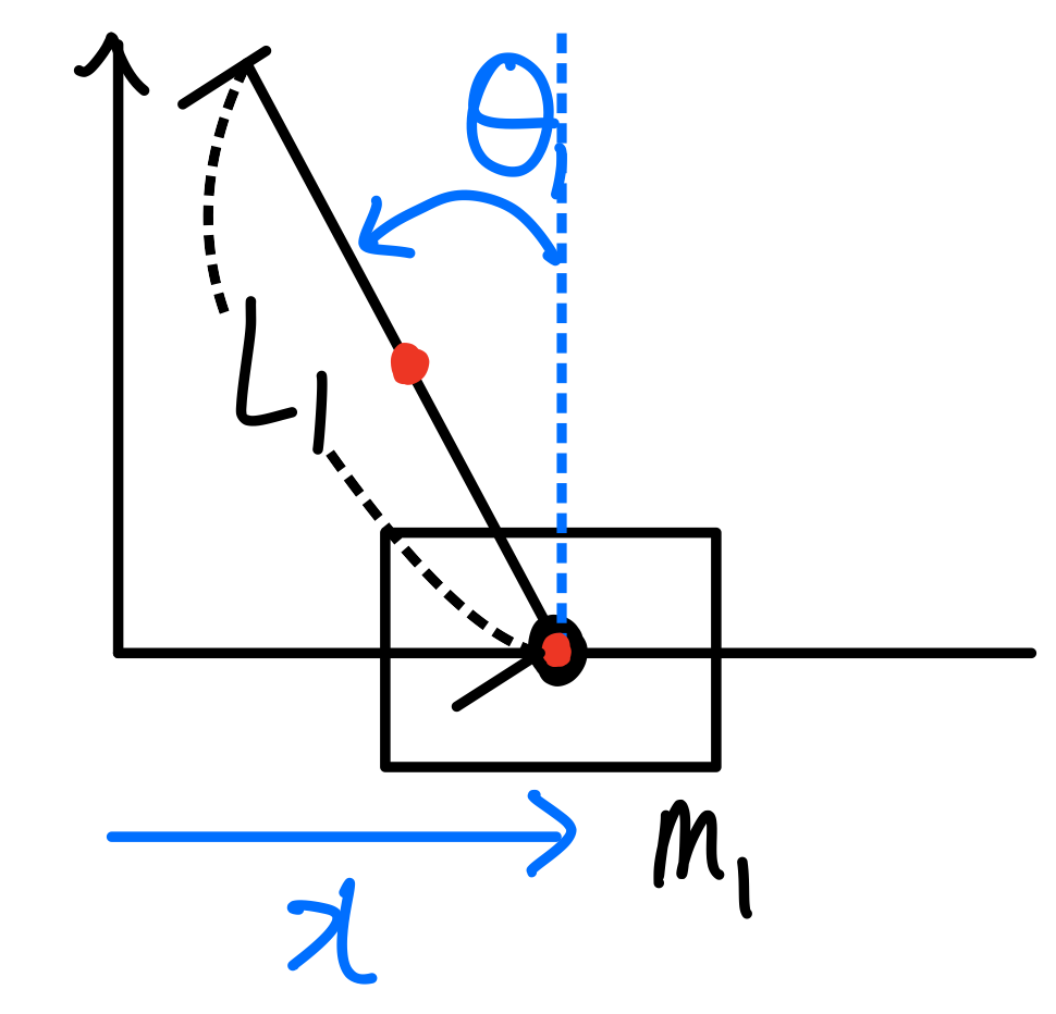
Consider a pendulum mounted on a cart, as illustrated in the following free body diagram:

To understand state feedback control in practice, let’s consider the example of a pendulum mounted on a cart. The following diagram illustrates the free body diagram of this system:

2. Equation of Motion

The nonlinear equation of motion for this system is derived using Lagrangian mechanics:

Where:

• \(m_0\) and \(m_1\) are the masses of the cart and pendulum
• \(l_1\) is the length of the pendulum
• \(\theta_1\) is the angle of the pendulum
• \(F\) is the force applied to the cart
• \(g\) is the acceleration due to gravity

You can find the detailed calculation in Day 3.

3. Linearization

To apply linear control techniques, we need to linearize the equation of motion. We do this by approximating the system behavior around the unstable equilibrium point where \(\theta_1 \approx 0\). Using small-angle approximations:

The linearized equation becomes:

4. State Space Representation

To convert the linearized equations into a state space representation, we isolate the accelerations \(\ddot{x}\) and \(\ddot{\theta}_1\):

We then express the system in state space form by defining the state vector \(x = [x_1, x_2, x_3, x_4]^T = [x, \theta_1, \dot{x}, \dot{\theta}_1]^T\):

5. Our system

For a specific system with \(m_0 = 0.0027\), \(m_1 = 0.0378\), and \(l_1 = 0.14\), we get:

The output equation is:

Thus, our state space matrices \(A\), \(B\), \(C\), and \(D\) are:

6. Checking Controllability in MATLAB

Controllability is a crucial property for implementing state feedback control. MATLAB provides simple functions to check the controllability of a system:

1. Create the state-space model:

   sys = ss(A, B, C, D);
   

2. Compute the controllability matrix:

   Co = ctrb(sys); // If you defined a system
   Co = ctrb(A, B); // If you have the matrix A and B
   

3. Check the rank of the controllability matrix:

   rank_Co = rank(Co);
   

4. Compare the rank with the number of states. If they’re equal, the system is controllable.

7. Implementing Pole Placement in MATLAB

The pole placement method is used to design the state-feedback gain matrix K for desired closed-loop pole locations. MATLAB’s place function simplifies this process:

a) Using the place Function

The basic syntax is:

K = place(A, B, P)

Where:

• A and B are the system matrices from the state-space model
• P is a vector containing the desired closed-loop pole locations
• K is the resulting state-feedback gain matrix

8. Bang-Bang Controller

For the swing-up phase of the inverted pendulum control, a Bang-Bang controller can be effective. This simple strategy applies maximum force in either direction based on the pendulum’s state.

a) Control Strategy

The Bang-Bang control law for the inverted pendulum is:

Where:

• \(u\) is the control input (force applied to the cart)
• \(u_{max}\) is the maximum allowable control input
• \(\dot{\theta}\) is the angular velocity of the pendulum

b) Switching Function

The switching function is based on the pendulum’s angular velocity:

c) Control Logic

• When \(\dot{\theta} > 0\) (clockwise motion), apply negative force to the cart.
• When \(\dot{\theta} < 0\) (counterclockwise motion), apply positive force to the cart.

This strategy opposes the pendulum’s motion, adding energy to the system and causing the pendulum to swing with increasing amplitude until it approaches the upright position.

III. Simulink Implementation

1. Overall System

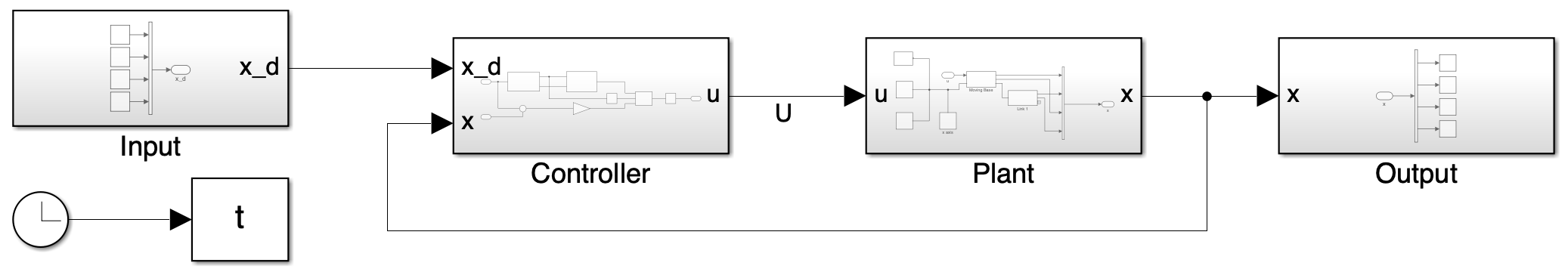
This closed-loop block diagram illustrates the interaction between our controller and the inverted pendulum (our plant). The controller processes the system state and generates a control signal, which in turn affects the pendulum’s behavior.

2. Input & Output Block

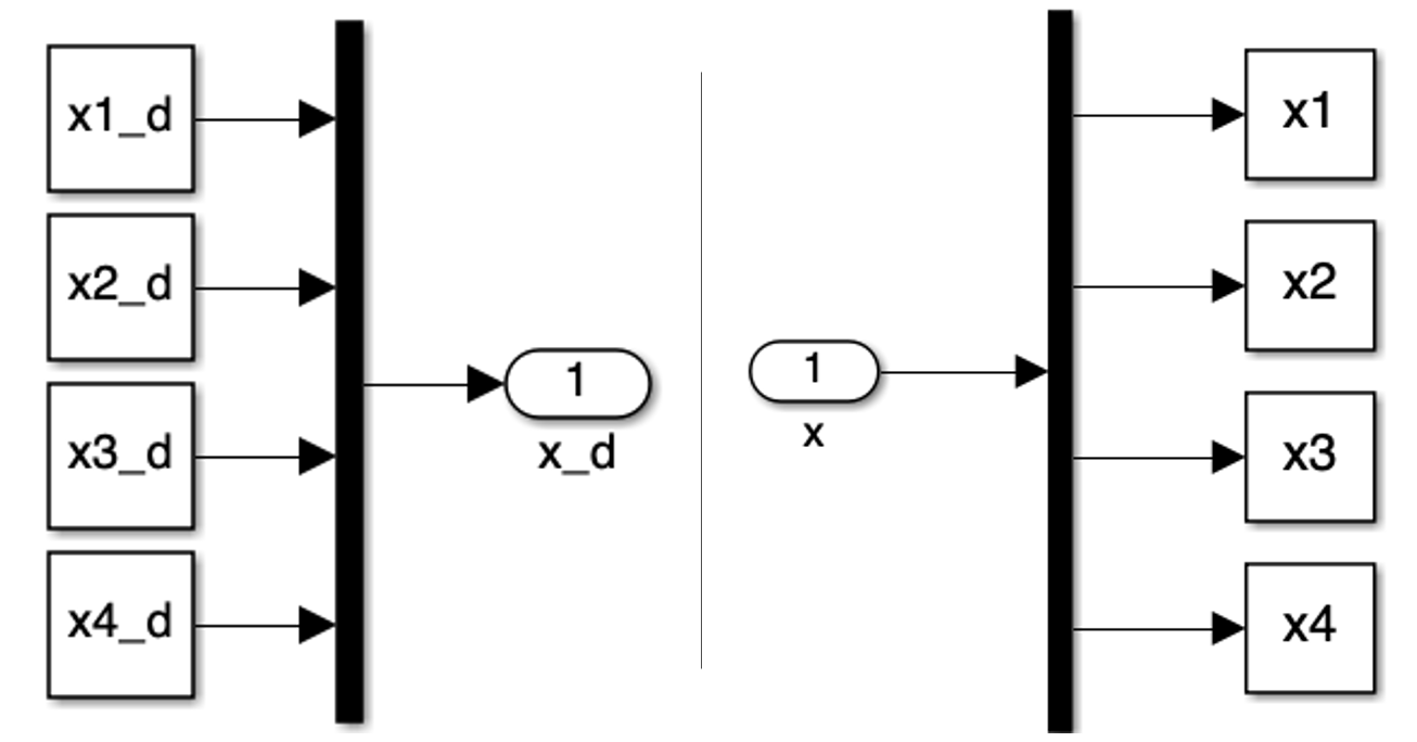
Our system state is characterized by four variables:

• \(x_1 = x\): The cart’s position
• \(x_2 = \theta\): The pendulum’s angle
• \(x_3 = \dot{x}\): The cart’s velocity
• \(x_4 = \dot{\theta}\): The pendulum’s angular velocity

These states are consolidated into a single vector in the input block and disaggregated in the output block, facilitating efficient manipulation within our control loop.

3. Plant Block

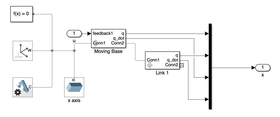
This block encapsulates the dynamics of our inverted pendulum system. It comprises a moving base (the cart) and the pendulum (link 1). The input \(u\) is applied exclusively to the moving base, which subsequently influences the pendulum’s motion.

4. Controller Block

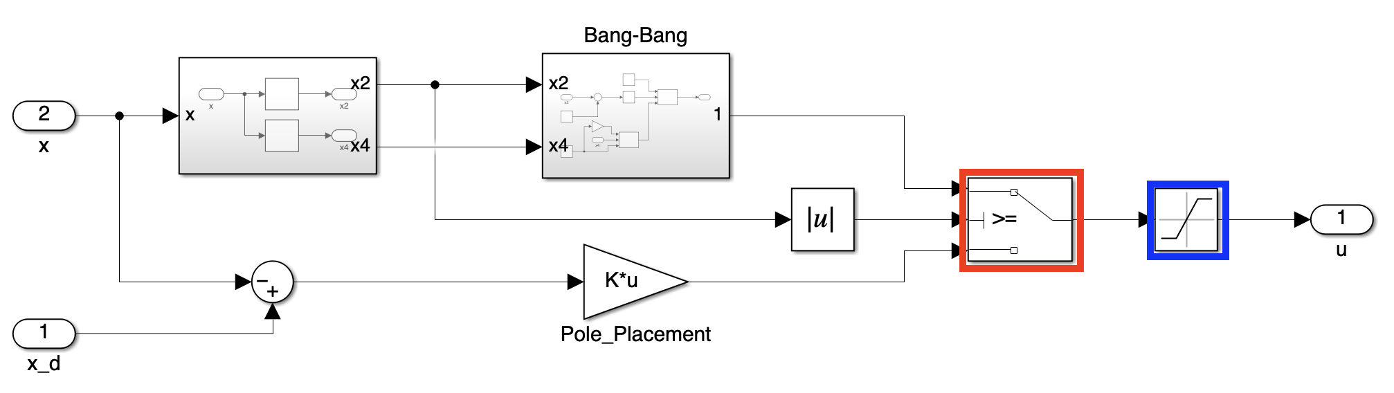
The controller is the core of our system, responsible for maintaining the pendulum’s upright position and stability. Let’s break down its key components:

• Red box (Switch): This block determines which feedback value will be chosen based on the angular displacement of link 1. Stabilization feedback is applied when the angular displacement is between \(-30^{\circ} < \theta < 30^{\circ}\). Otherwise, Swing-Up control feedback is applied.
• Blue box (Saturation): This block limits the feedback’s magnitude.

The controller switches to stabilization control when the pendulum angle is between -30° and 30° from vertical. The maximum control force is limited to 0.45 N.

5. Bang-Bang Block

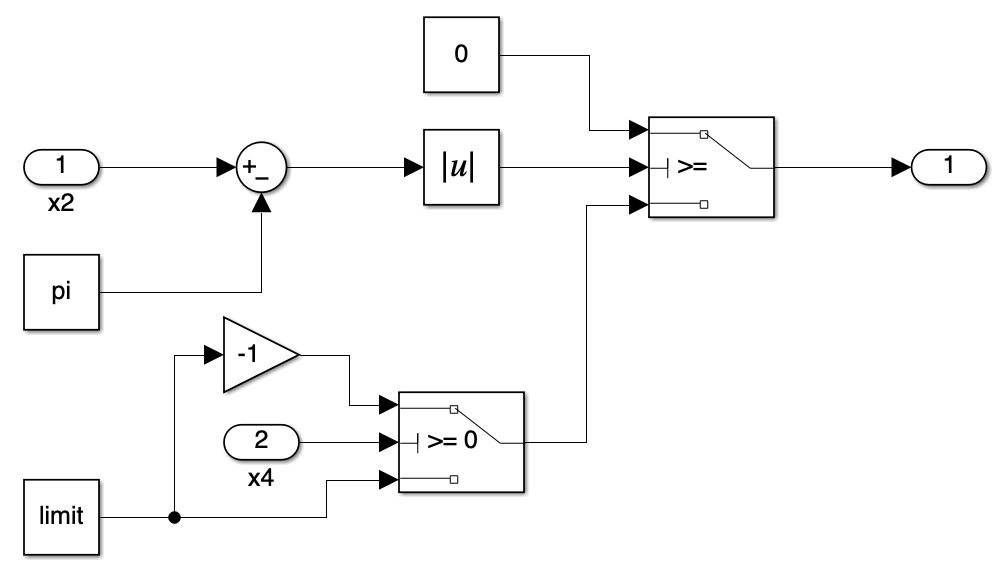
For swing-up control, we employ a bang-bang control strategy. This simple yet effective approach is used to bring the pendulum from its downward position to near the upright position, where the state feedback controller can then take over for stabilization.

The bang-bang control block determines the control input based on the pendulum’s angular velocity. It applies the maximum force in either the positive or negative direction, depending on the sign of the angular velocity. This creates a pumping effect that increases the pendulum’s energy, causing it to swing up.

IV. Simulation

For our simulation, we aimed to create a critically damped system where all poles are positioned on the real axis of the s-plane. However, due to limitations of MATLAB’s place function, we had to choose poles with multiplicity smaller than rank(B). Since the rank of B is 1, we selected poles with a 0.002 gap, such as -0.000, -0.002, -0.004, -0.006. This approach allowed us to create a system very close to critically damped while satisfying the constraints of the place function.

1. Tracking

a) Initial State: \(x = 0, \theta = 5^{\circ}\)

we first tested with a small initial angle of \(5^{\circ}\) in the initial state. For this small region, linearization was effective and the linear controller could manage the system well. As the poles move farther from the origin, the response becomes faster. The results are shown in Videos 1 - 4 and Figures 7 - 8.

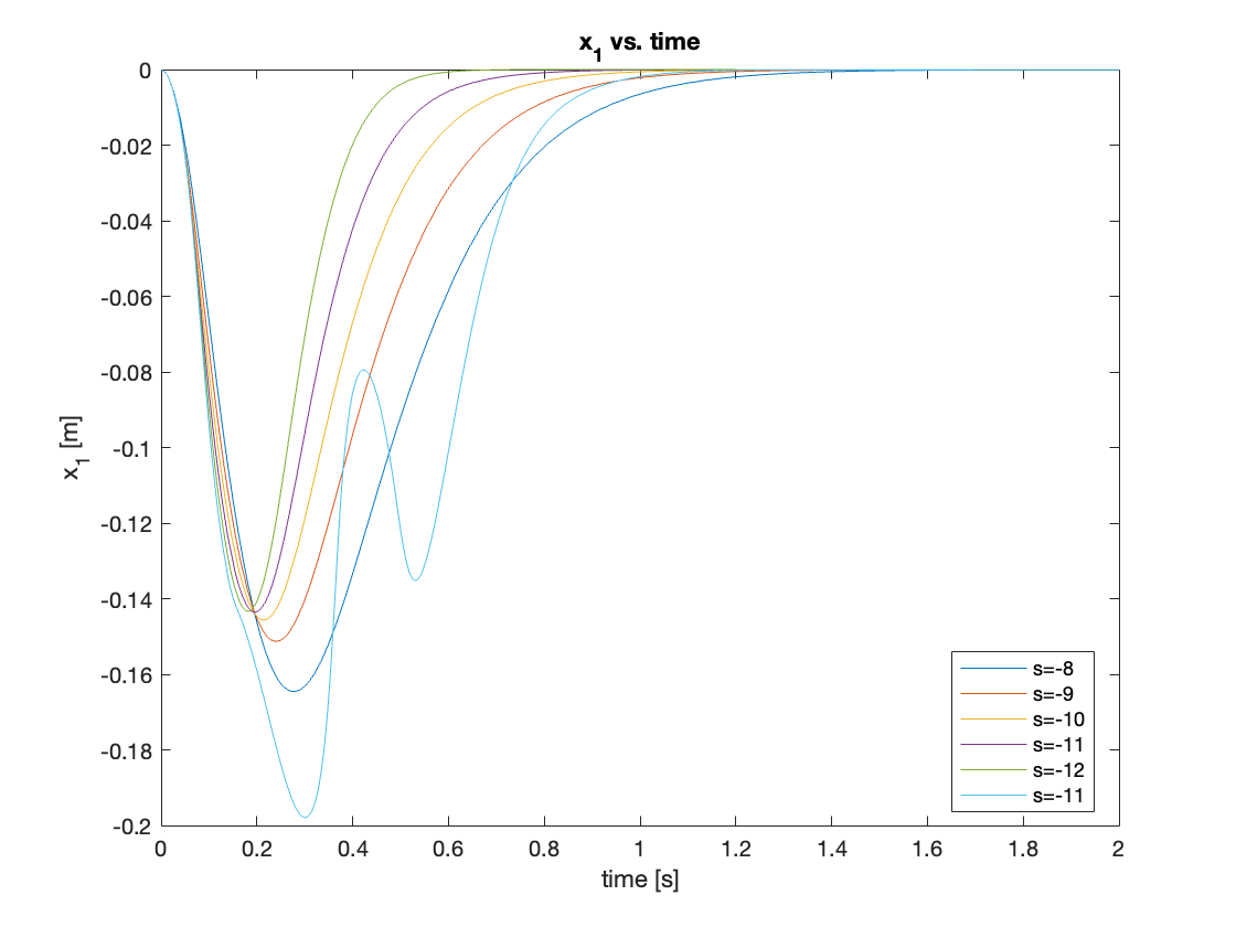
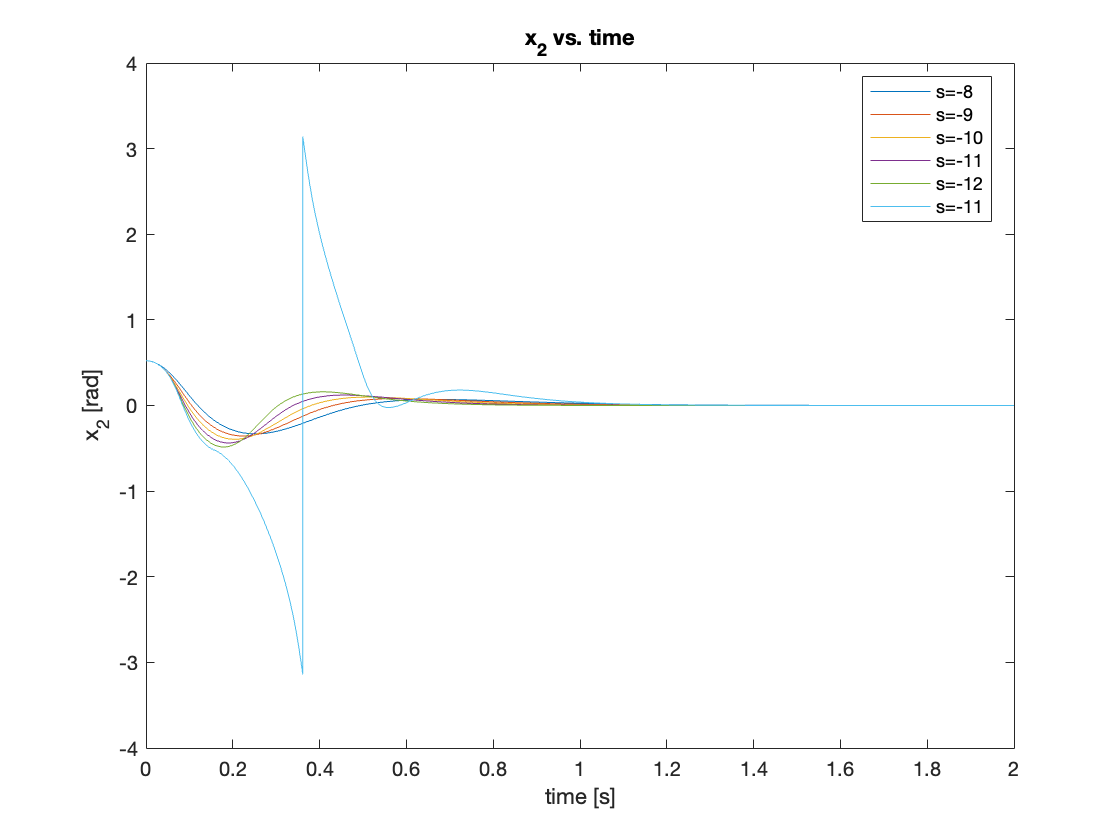
b) Initial State: \(x = 0, \theta = 30^{\circ}\)

Next, we increased the initial angle to \(\theta = 30^{\circ}\). Compared to the \(5^{\circ}\) initial angle, two different behaviors were observed:

1. The controller with the smallest pole magnitude (s = -1) couldn’t generate feedback large enough to raise the pendulum, resulting in failure to stabilize.
2. The controller with the largest pole magnitude (s = -15) initially lost some control, showing worse performance compared to the controller with poles at s = -10.

The results are shown in Video 5 and Figures 9 - 10.

Through iterative optimization, we found that the controller showed the best performance for \(\theta = 30^{\circ}\) when the poles are at \(s = -12\). The comparisons are shown in Figures 11 and 12.

c) Initial State: \(x = 0, \theta = 90^{\circ}\)

we increased the initial angle further to \(90^{\circ}\), allowing the swing-up controller to come into play. We tested poles at \(s = [-10, -12, -15, -18]\). Contrary to expectations, the controller with \(s = -15\) showed the best performance. This highlights a limitation of the pole placement method: the optimal controller varies depending on initial states. The results are shown in Video 6 and Figures 13 and 14.

d) Initial State: \(x = 0, \theta = 150^{\circ}\)

Issues arose when the initial angle reached \(150^{\circ}\). The system was stable only for a small range of pole positions from \(s = -3\) to \(s = -10\). The results are shown in Video 7.

e) Initial State: \(x = 0, \theta = 180^{\circ}, F = 0.1N\)

A similar problem occurred when applying a small force (0.1N) to the stable position (\(\theta = 180^{\circ}\) ). The results are shown in Video 8.

The issues observed in sections d) and e) may result from the transition between the Bang-Bang controller and the State Feedback Controller. If a pendulum is pushed by a user and loses its position, it could revolve very quickly. When the pendulum’s speed is high, the swing-up control law continues to accelerate the pendulum. As both acceleration and speed increase, the state feedback controller may fail to stabilize the system. This can cause the pendulum to rotate continuously, potentially leading to motor malfunction. Furthermore, finding the optimal controller parameters for these edge cases proves to be challenging.

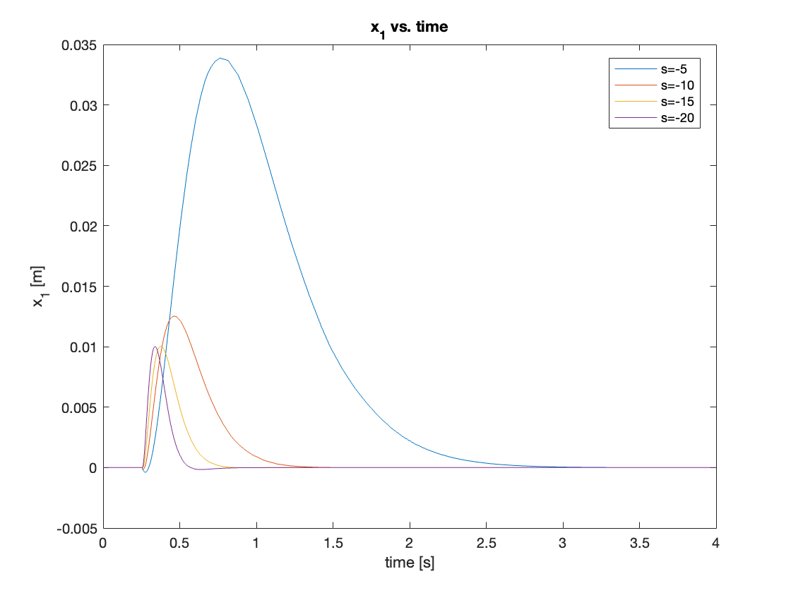
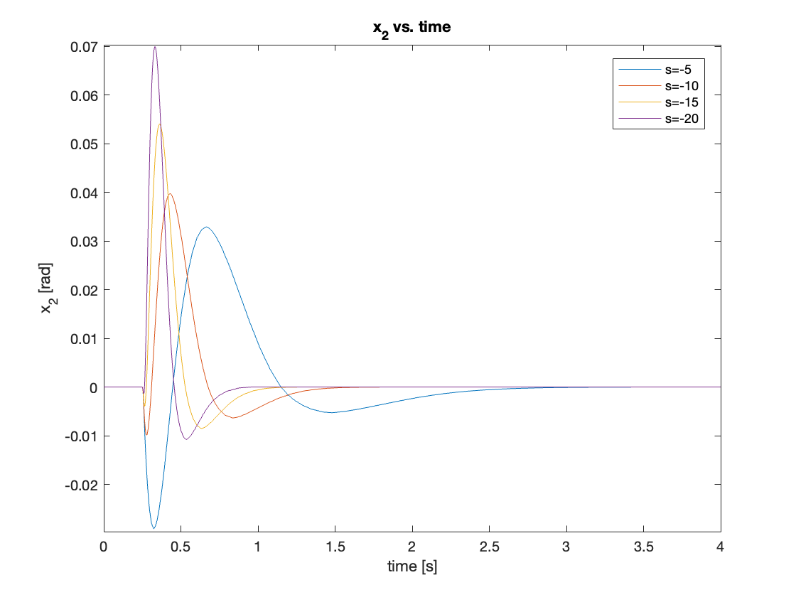
2. Regulation

a) Disturbance \(F = 0.1N\)

The regulation with small disturbance showed similar behavior to the tracking with small initial angle. The controller’s performance improves as the magnitude of poles increases. In this simulation, we used \(s = [-5, -10, -15, -20]\). The results are shown in Video 9 and Figures 15 and 16.

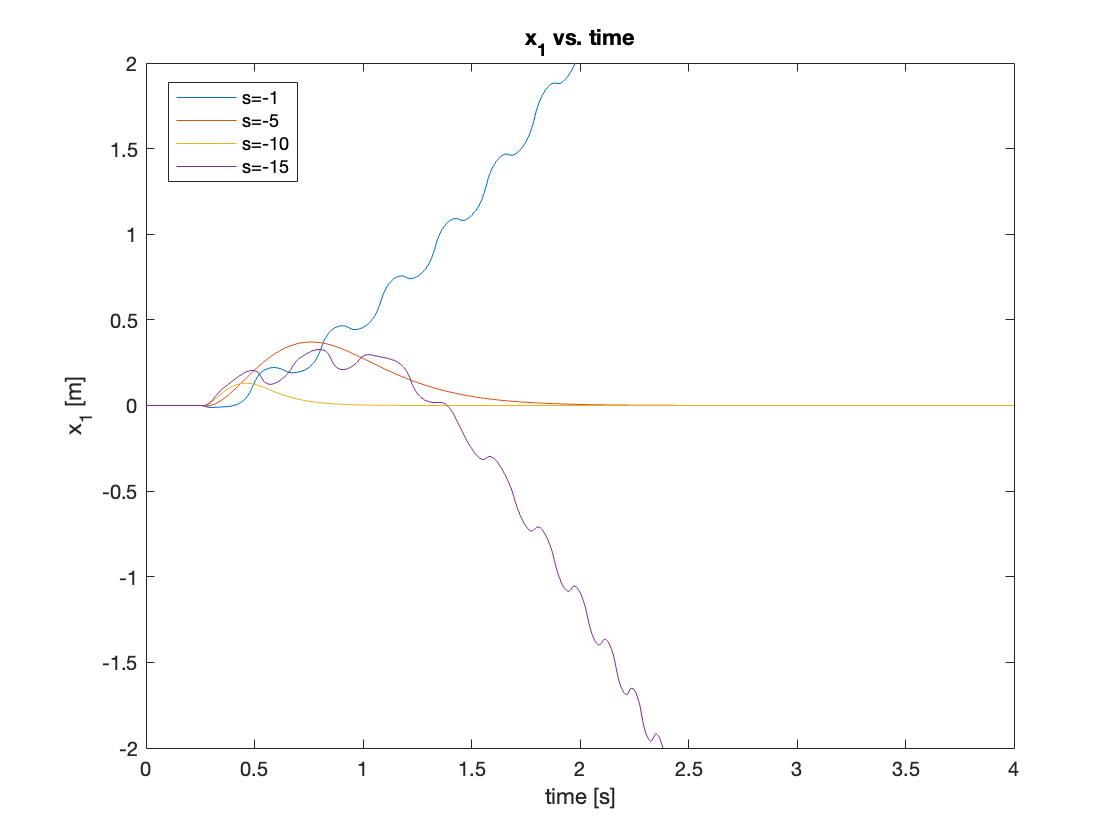
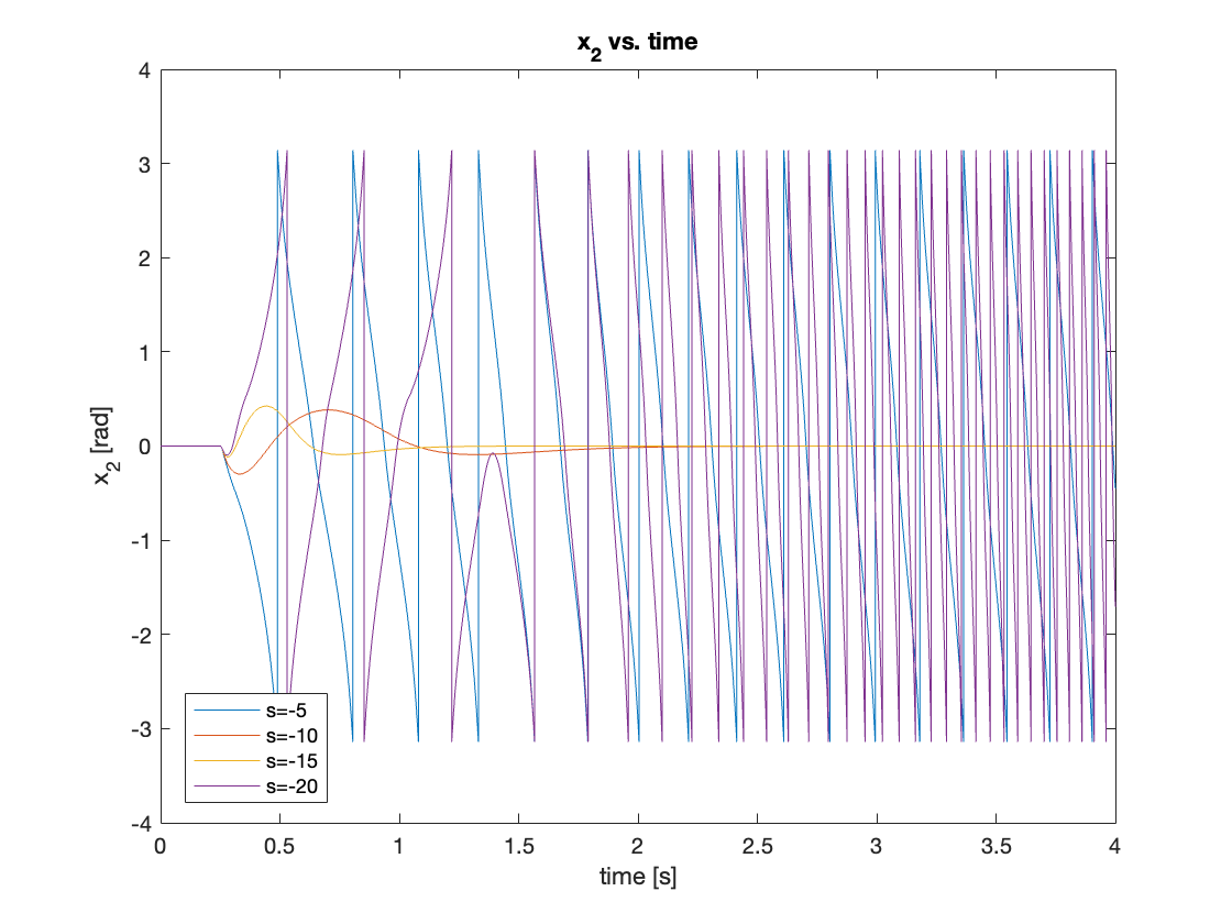
b) Disturbance \(F = 1N\)

Lastly, we simulated with a disturbance of 1N and found that if the pendulum moves beyond its linearized region \([-30^{\circ} \leq \theta \leq 30^{\circ}]\), the system becomes unstable. The reason for this was similar to the issue observed in the tracking simulation with large initial angles. When the pendulum’s speed is high, the swing-up control law continues to accelerate the pendulum. As both acceleration and speed increase, the state feedback controller may fail to stabilize the system.

For this simulation, we tested four cases, from small to large pole positions: \(s = [-1, -5, -10, -15]\). Similar to the large initial angle tracking, we found a sweet spot that can successfully regulate the system. Smaller pole magnitudes induced behavior similar to understeering, while bigger pole magnitudes led to oversteering. The results are shown in Video 10 and Figures 17 - 18.

3. Conclusion

Based on the simulations, we concluded that the best pole placement for this system is at \(s = -10\). The controller with this pole position demonstrated good tracking and regulation performance with short settling times. However, even this controller could not regulate the system when the disturbance exceeded 2N, as shown in Video 11 and Figure 19.

V. Conclusion and Moving Forward

Through our exploration of state feedback control for the inverted pendulum system, we’ve gained valuable insights into both the strengths and limitations of the pole placement method and Bang-Bang control. Our simulations demonstrated the effectiveness of these approaches within certain bounds, but also revealed challenges when dealing with large disturbances or initial conditions.

Based on these findings, our next steps will focus on implementing more advanced control strategies to address the limitations we’ve encountered:

1. LQR Controller for Stabilization: we will implement a Linear Quadratic Regulator (LQR) controller, which can be seen as an upgraded version of the pole placement method. LQR offers several advantages:
   • It provides a systematic way to find the optimal feedback gain matrix.
   • It allows us to balance the trade-off between control effort and state regulation through the Q and R matrices.
   • It often results in more robust control compared to simple pole placement.

   By implementing LQR, we aim to achieve better stabilization performance, especially for larger initial angles around the upright position.

2. Energy Shaping Control for Swing-Up: To improve upon the Bang-Bang control used for swing-up, we will implement Energy Shaping control. This method offers several benefits:
   • It provides a smoother control action compared to Bang-Bang control.
   • It explicitly considers the system’s energy, making it well-suited for the swing-up task.
   • It can potentially provide a more reliable transition to the stabilization controller.

   With Energy Shaping control, we hope to achieve more consistent swing-up performance and a smoother handover to the stabilization controller.

These advancements should address several of the limitations we observed:

• The sensitivity to pole placement that we encountered should be mitigated by the LQR’s systematic approach to gain selection.
• The challenges in transitioning from swing-up to stabilization control should be reduced with the more sophisticated Energy Shaping method.
• The overall robustness of the system should improve, potentially allowing us to handle larger disturbances and a wider range of initial conditions.

In our next update, we’ll dive into the theory behind LQR and Energy Shaping control, implement these methods for our inverted pendulum system, and compare their performance against our current pole placement and Bang-Bang control strategies. We’re excited to see how these advanced techniques will improve our inverted pendulum’s behavior across various scenarios!

Stay tuned as we continue to push the boundaries of control for this fascinating nonlinear system!

You can find the Simulink model on my GitHub repository.