I. Introduction

In this post, we’ll explore two advanced control techniques: Linear Quadratic Regulator (LQR) for stabilization and Energy Shaping for swing-up control of an inverted pendulum system.

1. Linear Quadratic Regulator (LQR)

The LQR is a fundamental control strategy used in control systems engineering to optimally regulate the behavior of a linear dynamical system. It minimizes a quadratic cost function that balances tracking performance and control effort.

a) Principles of LQR

1. System Dynamics: LQR is designed for systems described by linear differential equations:

   \[\dot{x} = Ax + Bu \tag{1}\]

   where \(x\) is the state vector, \(u\) is the control input, and \(A\) and \(B\) are matrices defining the system dynamics.

2. Cost Function: LQR aims to minimize:

   \[J = \int_0^{\infty} (x^T Q x + u^T R u) \, dt\tag{2}\]

   Here, \(Q\) and \(R\) are weighting matrices. \(Q\) should be positive semi-definite, and \(R\) positive definite, prioritizing state precision and control effort respectively.

   • Matrix \(Q\) - State Cost Matrix:
     • Purpose: Weighs the state errors, penalizing deviations from desired states.
     • Properties: Positive semi-definite to ensure non-negative cost for state errors.
     • Effect: Higher values prioritize accuracy in corresponding state variables.
   • Matrix \(R\) - Control Effort Cost Matrix:
     • Purpose: Weighs the control effort, penalizing excessive use of control inputs.
     • Properties: Positive definite to ensure all control efforts have a positive associated cost.
     • Effect: Lower values can lead to more aggressive control actions; higher values promote conservatism.

3. Optimal Control Law: The solution is a linear control law:

   \[u = -Kx \tag{3}\]

   where \(K\) is the gain matrix calculated using the Riccati equation.

4. The Riccati Equation: The Riccati equation is a differential equation crucial for determining the LQR gain matrix \(K\):

   \[\dot{P} = A^T P + PA - PBR^{-1}B^T P + Q \tag{4}\]

   In this equation, \(P\) is a matrix that solves the Riccati equation. Once \(P\) is determined, the optimal gain matrix \(K\) can be computed as:

   \[K = R^{-1}B^T P \tag{5}\]
   • Matrix \(P\) - Solution to the Riccati Equation:
     • Purpose: Balances the trade-off between tracking performance and control effort in the cost function.
     • Properties: Symmetric positive definite.
     • Role: Directly influences the gain matrix \(K\), dictating the control action.

   Solving the Riccati equation enables the calculation of the necessary feedback gains to minimize the cost function \(J\), effectively aligning the system’s behavior with the desired performance objectives while minimizing control effort. This makes LQR a powerful tool for achieving optimal control in linear systems.

b) Advantages of LQR

• Optimality: Provides optimal control for defined cost function and system dynamics.
• Robustness: Offers robustness to model uncertainties and disturbances within linear framework.
• Simplicity: Once \(K\) is computed, the linear control law is straightforward to implement.

c) Limitations

• Model Dependence: Requires accurate linear model, limiting effectiveness for nonlinear systems.
• Tuning Complexity: Choosing appropriate \(Q\) and \(R\) matrices can be complex and requires domain knowledge.

d) Applications

LQR finds wide application in fields requiring optimal control for linear systems:

1. Aerospace engineering: Aircraft flight control, spacecraft attitude stabilization
2. Automotive systems: Active suspension, cruise control optimization
3. Robotics: Robot arm positioning, quadcopter stabilization
4. Industrial processes: Chemical reactor regulation, manufacturing automation
5. Power systems: Electrical grid control, wind turbine optimization
6. Consumer electronics: Hard disk drive positioning, camera stabilization

2. Energy Shaping

While LQR control is effective around an equilibrium point, swinging up a pendulum requires handling larger deviations from equilibrium. For this, we use Energy Shaping, which begins with partial feedback linearization of the equation of motion.

a) Principles of Energy Shaping

1. System Energy: Based on modifying the system’s energy function to achieve desired behavior.

2. Potential Energy Shaping: Alters the potential energy landscape to create equilibrium at desired points.

3. Kinetic Energy Shaping: Modifies the kinetic energy to influence system dynamics.

4. Interconnection and Damping Assignment: Adjusts system interconnections and adds damping for stability.

5. Lyapunov Stability: Ensures closed-loop stability by shaping energy functions as Lyapunov functions.

b) Advantages of Energy Shaping

• Physical Insight: Provides intuitive understanding of system behavior through energy concepts.
• Nonlinear Systems: Applicable to a wide range of nonlinear systems.
• Stability Guarantee: Ensures stability through proper energy function design.
• Robustness: Can offer robustness to certain types of uncertainties and disturbances.

c) Limitations

• System Knowledge: Requires detailed knowledge of system’s physical structure and energy properties.
• Mathematical Complexity: Can involve complex calculations for energy function derivation.
• Applicability: Not all systems have easily identifiable or modifiable energy functions.

d) Applications

Energy Shaping finds wide application in fields requiring control of complex, often nonlinear systems:

1. Robotics: Humanoid robot balance, manipulator control
2. Mechanical systems: Pendulum stabilization, vibration control
3. Aerospace: Spacecraft attitude control, helicopter stabilization
4. Power systems: Power converter control, microgrid stabilization
5. Biomechanics: Prosthetic limb control, exoskeleton systems
6. Marine systems: Ship stabilization, underwater vehicle control

II. Mathematical Modeling and Analysis

1. LQR

LQR design for the inverted pendulum on a cart begins with developing a linear state-space model.

a) Linearization of the System

The process to linearize the system (including Equation of Motion, Linearization, and State Space Representation) is explained in detail in Day 6. The resulting state-space matrices are:

b) Implementing LQR in MATLAB

Once the state-space model of your system is established, you can compute the LQR gain matrix using MATLAB:

K_LQR = lqr(A, B, Q, R);

This command utilizes MATLAB’s built-in lqr function, which requires the system’s matrices \(A\) and \(B\) along with the weight matrices \(Q\) and \(R\). The function returns the optimal gain matrix K_LQR.

2. Energy Shaping

Energy Shaping for the inverted pendulum on a cart focuses on explicitly modeling and modifying the system’s energy functions. This approach considers both the kinetic energy (from the cart’s translation and the pendulum’s rotation) and the potential energy (due to the pendulum’s position in the gravitational field).

a) Partial Feedback Linearization

Starting from Equation 11 in Day 6, we drive:

Applying feedback control, we set:

This results in the decoupling of the system:

Letting \(u = \ddot{x}^d\), we simplify this to:

Equation 11 is straightforward, allowing us to focus on handling Equation 12.

b) Energy Regulation Using Energy Shaping

The energy of the pendulum is expressed as:

At the equilibrium point (\(\theta_1 = 0, \dot{\theta}_1 = 0\)), the desired energy level is:

To stabilize the system, we compute the derivative of the energy error, \(\tilde{E}(\theta, \dot{\theta}) = E(\theta) - E^d\):

The control input is defined to stabilize the pendulum as:

This approach allows us to effectively swing up the pendulum using energy shaping, ensuring that the system is not only responsive but also stable under varying conditions.

III. Simulink Implementation

1. Overall System, Input/Output, Plant

The overall system, input/output, and plant blocks remain the same as in Day 6. For this and future posts, we will focus on updating only the Controller block.

2. Controller Block

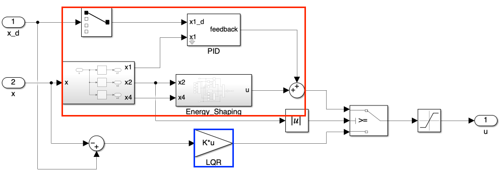
The controller block has been updated to incorporate LQR and Energy Shaping control:

• Red box (Energy Shaping): This component is responsible for the swing-up motion. Since Energy Shaping doesn’t account for the cart’s linear displacement, we’ve added a PID controller to manage the cart’s position.
• Blue box (LQR): This component is similar to the one used for the pole placement method, but now utilizes the feedback gain determined by the LQR method.

The controller switches between swing-up and stabilization control based on the pendulum’s angle:

• Swing-up control (Energy Shaping) is active when the pendulum angle is outside the range of ±30° from vertical.
• Stabilization control (LQR) takes over when the pendulum angle is within ±30° of vertical.

The maximum control force is limited to 0.45 N to prevent excessive actuation.

3. Energy Shaping Block

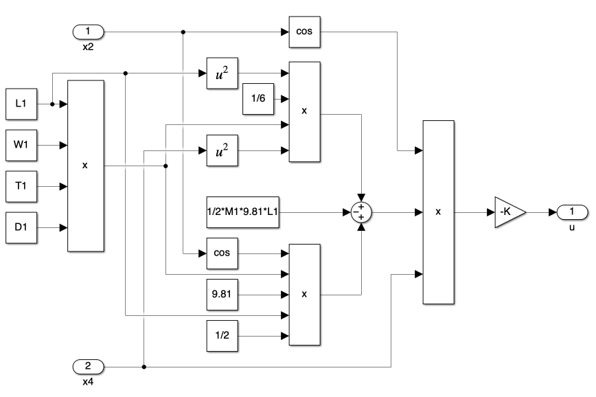
The Energy Shaping block implements the swing-up control strategy derived in Section we.B. It calculates the control input \(u\) based on the pendulum’s current state:

Where:

• \(k\) is a positive gain constant
• \(\theta\) is the pendulum angle
• \(\dot{\theta}\) is the angular velocity of the pendulum
• \(\tilde{E}(\theta, \dot{\theta})\) is the energy error (difference between current and desired energy)

This control law strategically injects or removes energy from the system to bring the pendulum to its upright position. The cosine term ensures that the control action smoothly transitions to zero as the pendulum approaches the vertical position, facilitating a seamless handover to the LQR controller for stabilization.

IV. Simulation

Tracking okay. Regulation 1N : Done by LQR 1.2N : Done by Bang-Bang + LAR (1 rotation) 1.3N : Done by Bang-Bang + LAR (3 rotation) 1.4 ~ 1.5N : Diverse, left way, due to LQR’s x1 correction 1.6N : Diverse, right way,

A. Energy Convergence and Controller Component Analysis

In this first simulation, we will demonstrate the effectiveness of the combined Energy Shaping and LQR control strategy for the inverted pendulum system. The simulation will focus on the full cycle of operation, from the pendulum’s initial position through swing-up and final stabilization in the upright position.

Key aspects to be analyzed:

1. Energy convergence during the swing-up phase
2. Transition between Energy Shaping and LQR control
3. Stabilization performance of the LQR controller
4. Contribution of each controller component to the overall system behavior

The simulation will start with the pendulum in different initial angles and run for 10 seconds to capture the complete motion. We will examine the system’s states and energy levels throughout this period to gain insights into the control strategy’s performance.

By analyzing the energy convergence and the role of each controller component, we aim to demonstrate how this approach achieves efficient swing-up and precise stabilization of the inverted pendulum system.

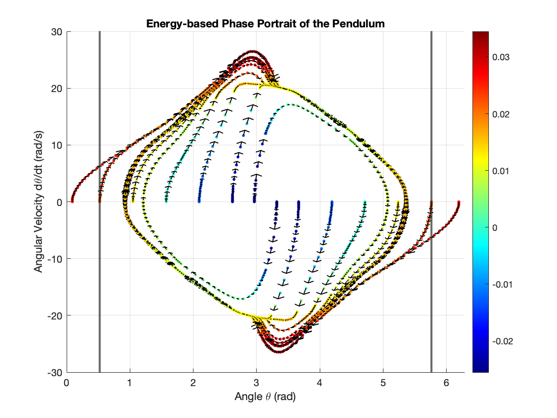
0. Uncontrolled System Behavior

Before applying any control strategies, it’s crucial to understand the natural behavior of the inverted pendulum system. In this section, we’ll examine how the cart-pendulum system behaves differently according to various initial states when there is no control input applied.

To observe this, we disconnected all controllers from the input signal, effectively leaving the system uncontrolled. Figure 3 illustrates the phase portrait of the pendulum for different initial conditions.

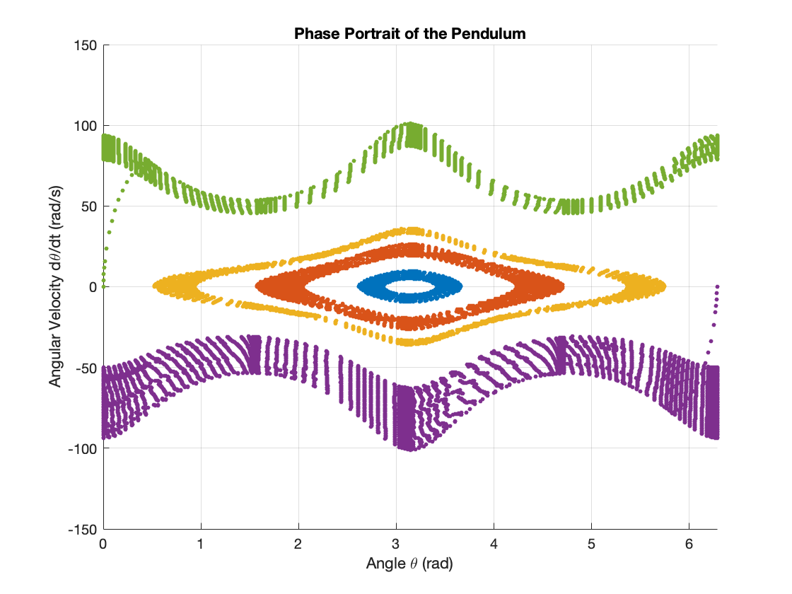
Key observations from this analysis:

1. Stable Limit Cycles: Some initial states result in stable limit cycles. These represent oscillations where the pendulum swings back and forth with consistent amplitude, neither gaining nor losing energy over time.

2. High Energy States: Other initial states, particularly those with higher initial energy, exhibit different behavior. These trajectories may:
   • Result in the pendulum completing full rotations
   • Show larger amplitude oscillations
   • Potentially lead to unstable or chaotic motion
3. Energy Conservation: In the absence of friction or other dissipative forces, the total energy of the system should remain constant. This is reflected in the closed orbits in the phase portrait.
   • However, due to the limitations of the ODE solver (DAESSC), our results appear slightly different from the ideal limit cycles shown in Figure 4.
4. Sensitivity to Initial Conditions: The wide variety of trajectories demonstrates the system’s sensitivity to initial conditions, a characteristic of nonlinear systems.

Reference: Winter, O., & Murray, C. (1997). Resonance and chaos: we. First-order interior resonances. Astronomy and Astrophysics, 319, 290-304.

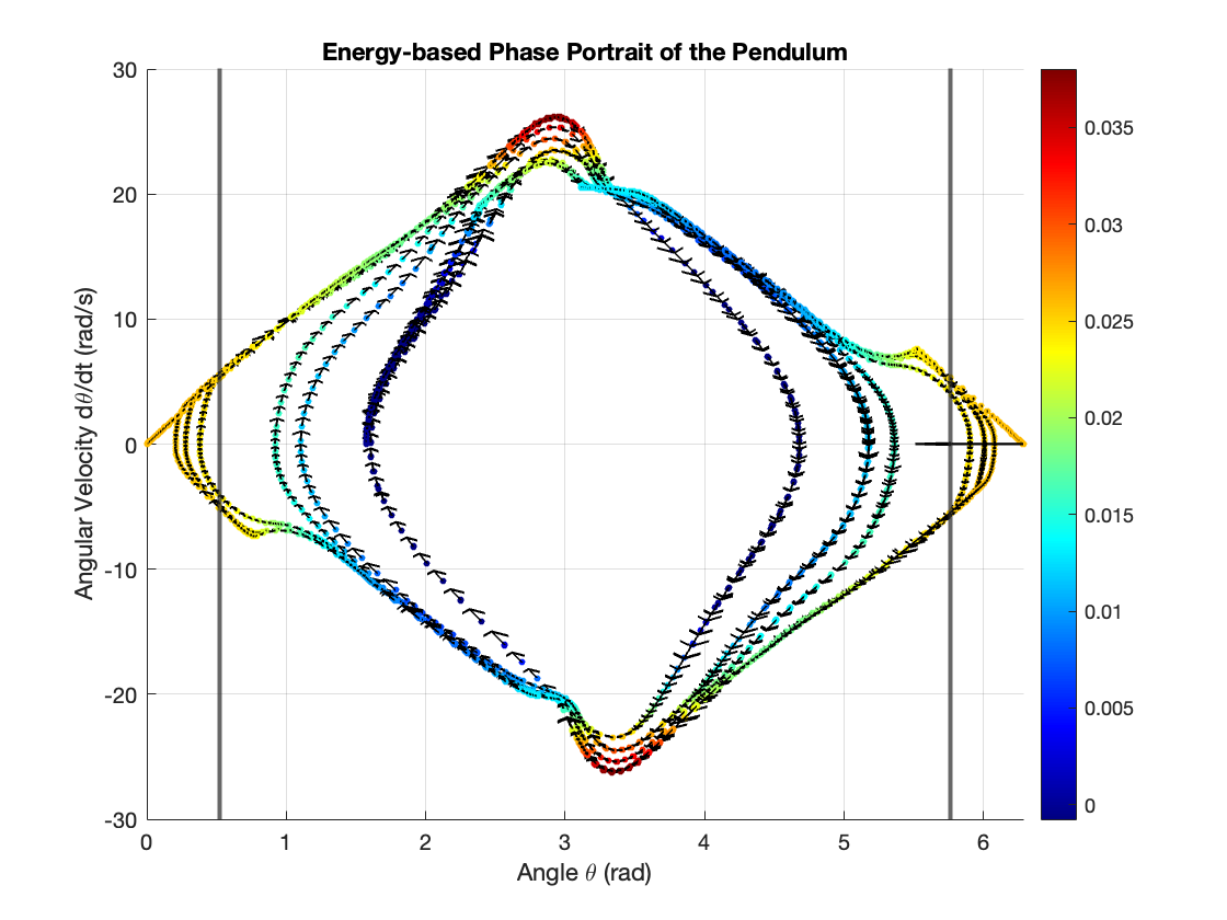
1. Using Energy Shaping Controller Only

In this section, we’ll isolate the Energy Shaping Controller to understand its behavior and effectiveness in swinging up the pendulum.

a) Fixed Gain \(K\), Varying Initial Condition \(\theta_0\)

Here, we’ll keep the controller gain \(K\) constant and observe how the system responds to different initial angles of the pendulum. This allows us to analyze the effect of the initial condition \(\theta_0\).

Figure 5 shows the simulations with different initial conditions when the gain is fixed at \(K = 10\). We tested initial angles \(\theta_0 = [\pm 5^{\circ}, \pm 30^{\circ}, \pm 60^{\circ}, \pm 90^{\circ}, \pm 120^{\circ}, \pm 150^{\circ}, \pm 170^{\circ} ]\). As observed, regardless of the starting position, all trajectories converge to a limit cycle. This demonstrates that if the system lacks sufficient energy, the controller provides energy to the system; conversely, if the system has excess energy, the controller removes energy from the system.

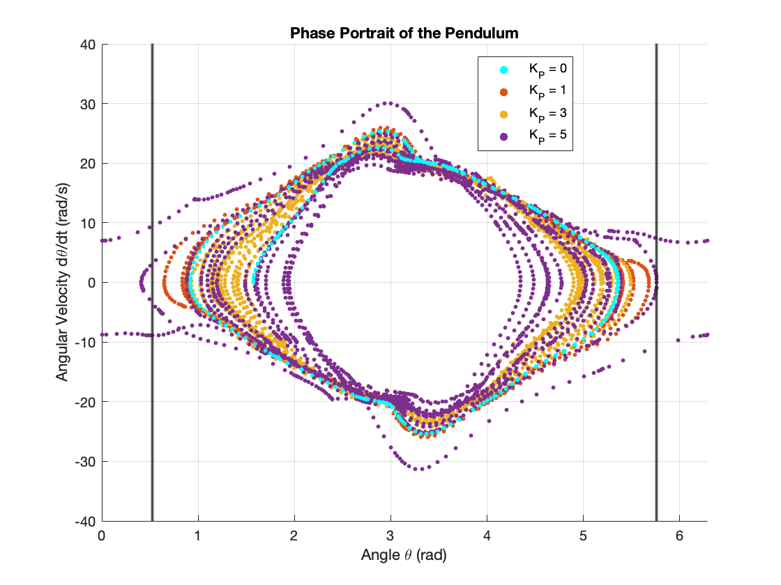
b) Varying Gain \(K\), Fixed Initial Condition \(\theta_0\)

In this part, we fix the initial pendulum angle and vary the controller gain \(K\) to examine its effect on system performance.

For this simulation, we set the initial angle to \(\theta_0 = 90^{\circ}\) and varied the gain using values \(K = [1, 5, 10, 20, 40, 80, 10^6]\). Figure 6 illustrates the results. As the gain \(K\) increases, the width of the limit cycle (range of angle) also increases. Interestingly, compared to the range of angle, the angular velocity is less affected by changes in gain.

2. Using Energy Shaping Controller with PID Controller

In this section, we combine the Energy Shaping Controller with a PID Controller to analyze their joint effect on the pendulum’s behavior. We fix the Energy Shaping gain at \(K = 10\) and the initial angle at \(\theta_0 = 90^\circ\), while varying the PID controller’s gains.

For the PID controller, we set the ratio of gains as \(K_P : K_I : K_D = 100 : 1 : 10\). Figure 7 illustrates the results of this combined control strategy.

Key observations from this analysis:

1. Higher PID gains generally reduce the range of pendulum angle, unless resonance occurs between the Energy Shaping and PID controllers.

2. The chosen Energy Shaping gain \(K = 10\) proves to be too small for effective control. With this gain, the pendulum fails to consistently reach the linearization region (outside the vertical lines in Figure 7).

3. Finding an optimal balance between the Energy Shaping and PID gains is crucial:

   • Too small an Energy Shaping gain \(K\) cannot effectively swing up the pendulum.
   • Too large an Energy Shaping gain \(K\) can overpower the PID controller, rendering it ineffective.

This analysis underscores the importance of carefully tuning both the Energy Shaping and PID controllers to achieve optimal performance in swinging up the pendulum and bringing it into the linearization region where LQR control can take over for final stabilization.

3. Combined All Together

In previous sections, we determined the minimum conditions for Energy Shaping and PID gains by examining the phase portrait. The goal was to swing up the pendulum sufficiently to reach the linearization region (\(-30^{\circ} < \theta < 30^{\circ}\)). Now, we’ll iteratively tune the LQR controller. To simplify the process, we’ll set \(K = 20\), \(K_P = 2\), \(K_I = 0.02\), and \(K_D = 0.2\), allowing us to focus on matrices \(R\) and \(Q\).

a) Varying Q, Fixed R

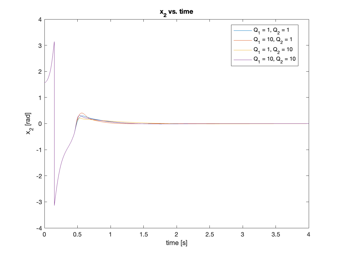
we’ll fix the control effort cost matrix \(R = 1\) to investigate the effect of the state cost matrix \(Q\). Video 1 and Figures 8 and 9 show that increasing \(Q_1\), which corresponds to the cart’s linear displacement, leads to faster \(x_1\) convergence. Similarly, increasing \(Q_2\) results in faster \(x_2\) convergence. The settling time seems to be most affected by \(x_1\). We tested four cases:

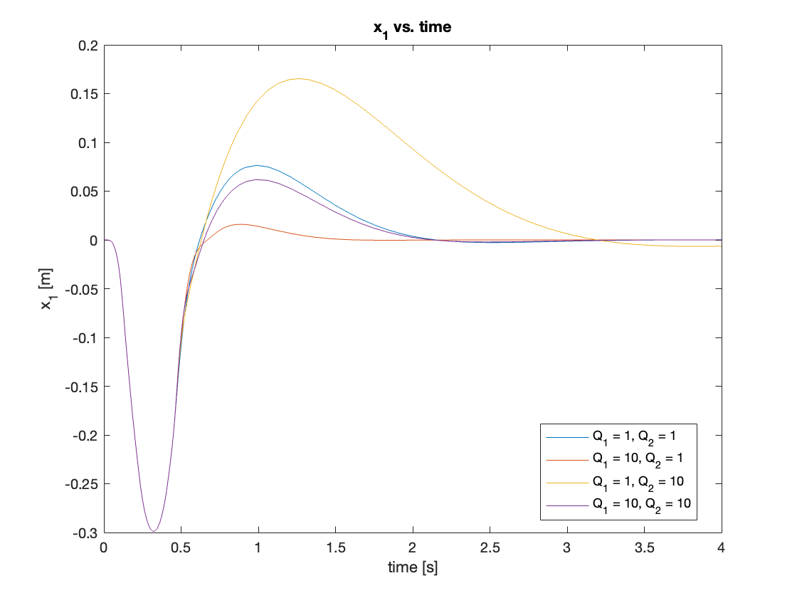
we then tested higher \(Q\) values:

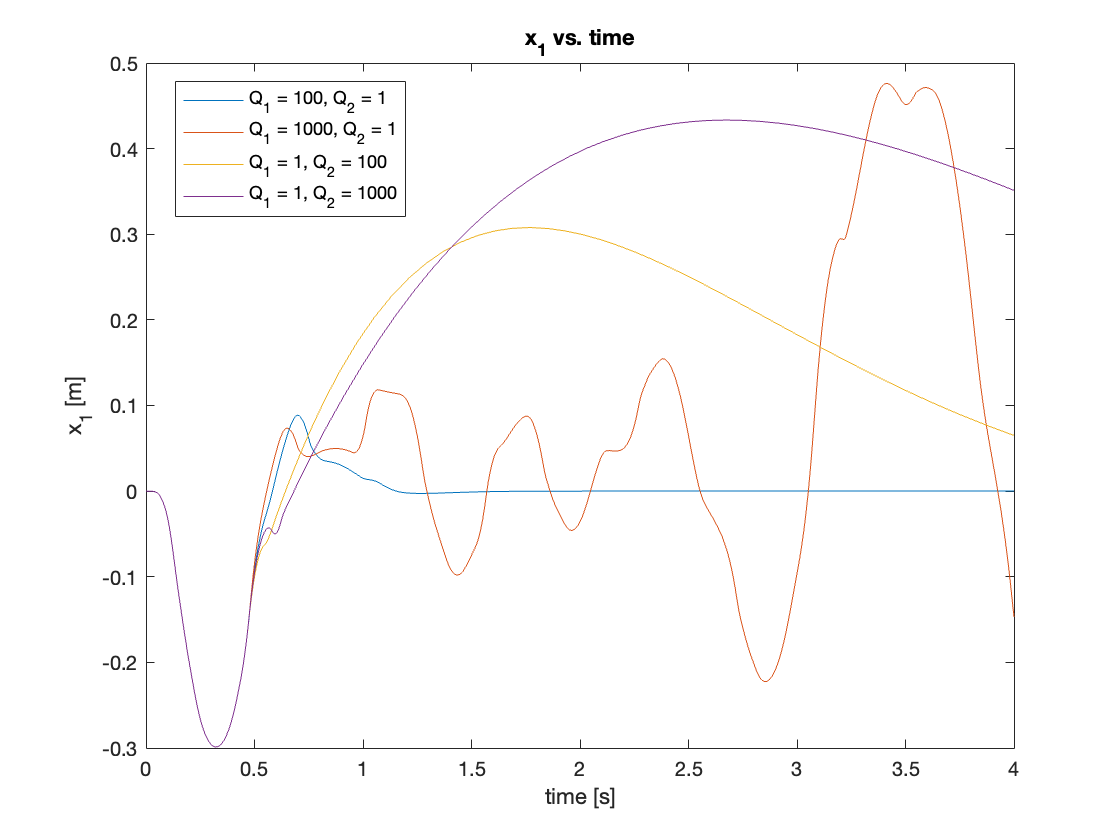
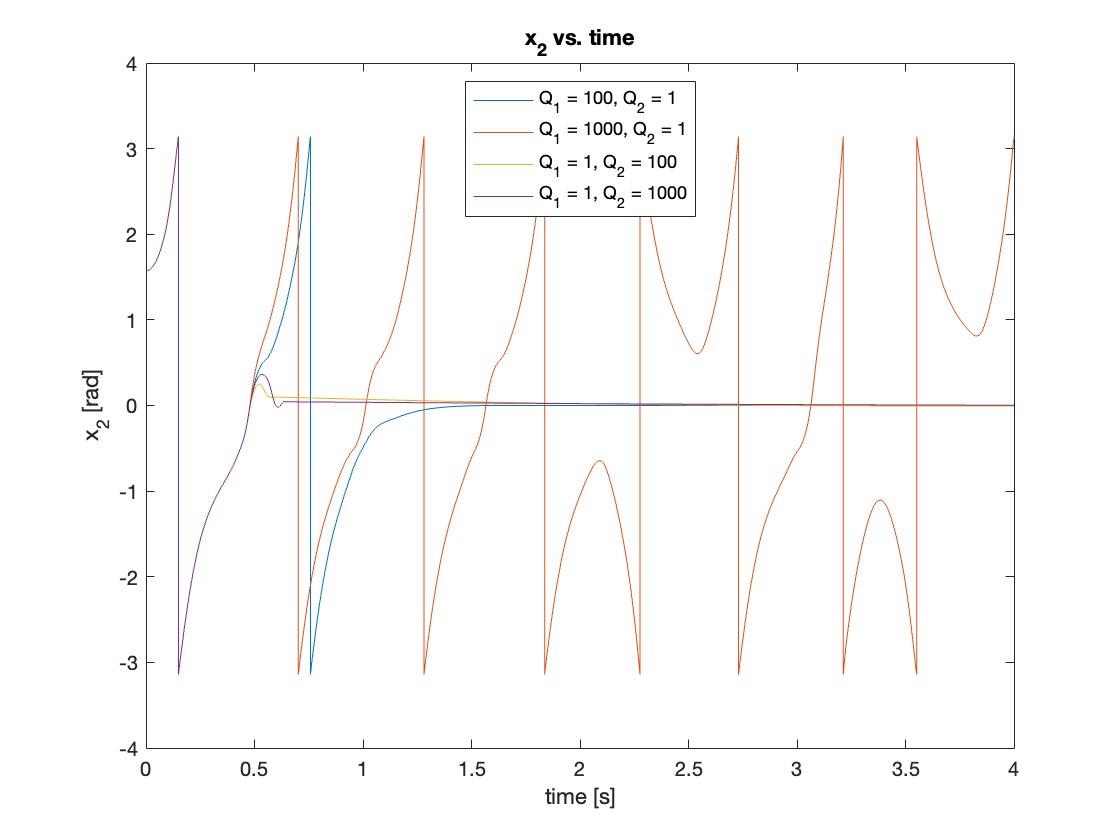
Video 2 and Figures 10 and 11 demonstrate that very high gains can lead to reduced performance or even system instability. This underscores the importance of iterative optimization through response inspection.

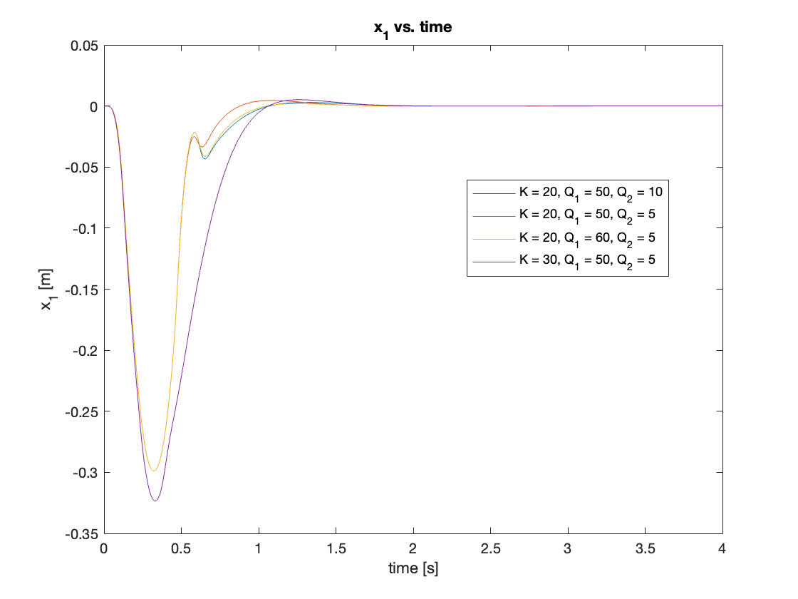
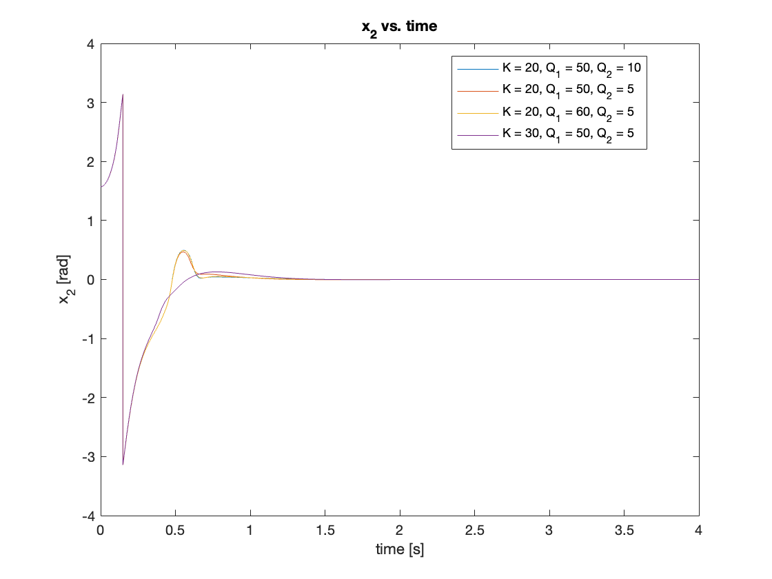
Through iterative optimization, we found that \(K = 20\), \(Q_1 = 50\), \(Q_2 = 5\) yielded the best performance, while \(K = 30\), \(Q_1 = 50\), \(Q_2 = 5\) produced the smoothest transient motion. Results are shown in Video 3 and Figures 12 - 13.

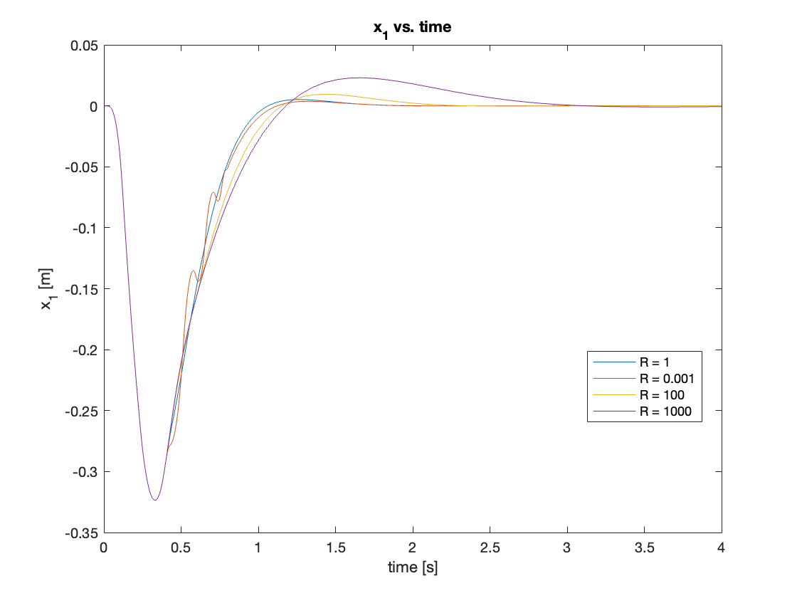
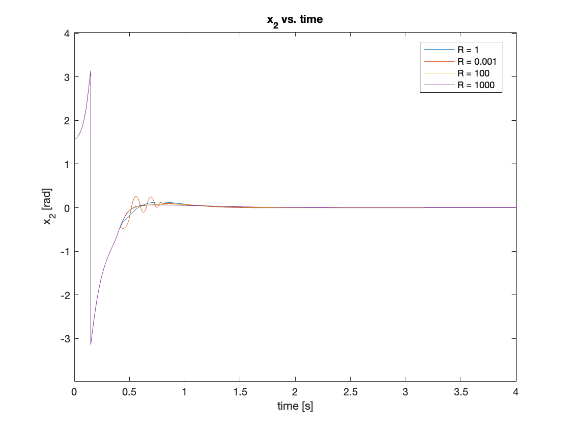
b) Fixed Q, Varying R

we tested \(R = [0.001, 1, 100, 1000]\) and observed that small \(R\) values lead to increased oscillation, while large \(R\) values result in slower settling times. Based on these observations, we decided to use \(R = 1\). Additionally, we set \(K = 20\), \(Q_1 = 50\), and \(Q_2 = 5\). This combination of parameters provided a good balance between performance and stability.

B. Tracking

After finalizing the controller tuning, we conducted tracking tests to evaluate the system’s performance. The results showed variable performance across different scenarios. In some cases, the controllers demonstrated excellent tracking capabilities, while in others, the system required more time to achieve the target state.

This inconsistency in tracking performance can be attributed to our tuning process, which primarily focused on a single initial condition. While effective for that specific case, this approach didn’t account for the full range of possible starting states our system might encounter.

To achieve more robust tracking performance, future work should focus on optimizing the controllers with various initial conditions. This approach would ensure that our system can handle a wide range of starting states, potentially leading to more consistent and reliable performance across different scenarios.

Video 4 and Figures 16 - 17 illustrate the results of our tracking simulations:

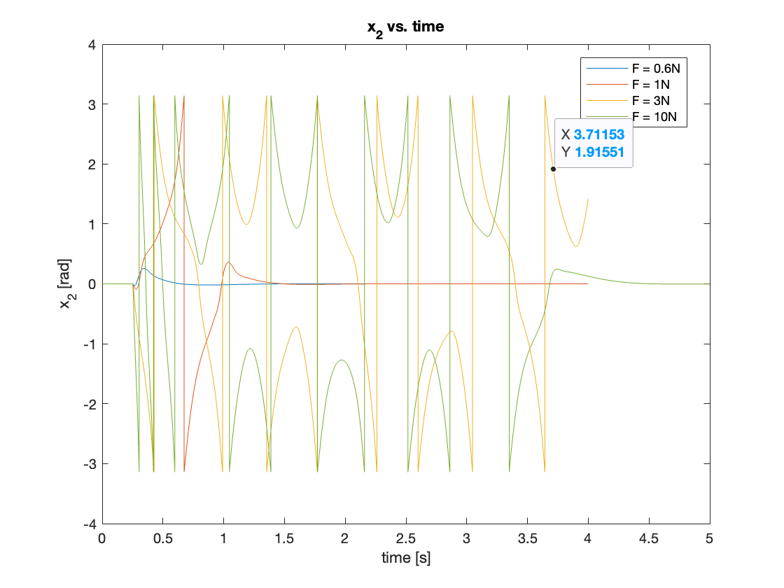
C. Regulation

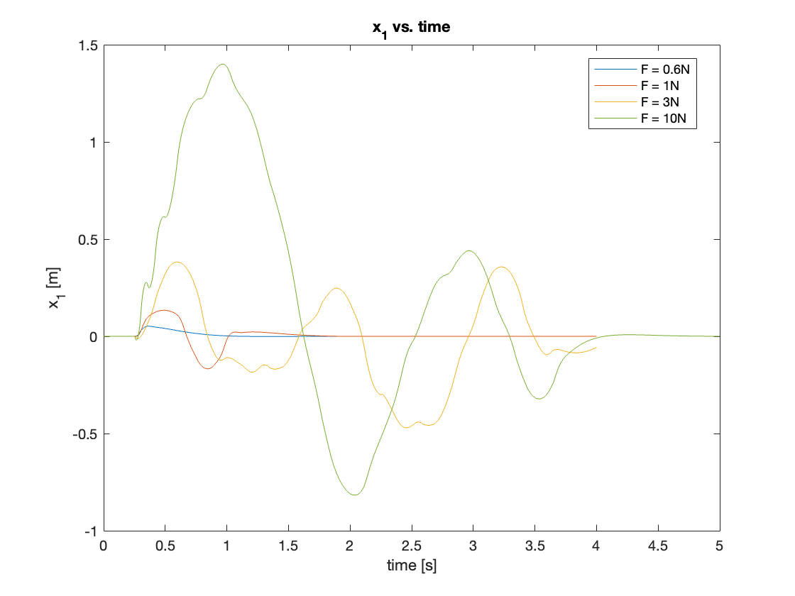
Lastly, we simulated regulation with disturbances of varying magnitudes. The system demonstrated different behaviors depending on the disturbance size:

1. For very small disturbances, the system easily regulated the position.
2. With larger disturbances that pushed the pendulum beyond a certain region, the system required one full rotation to return to the upright position.
3. In some cases, similar to the tracking scenarios, the controller failed to regulate the disturbance effectively.
4. For extremely large disturbances, the system took considerable time to achieve regulation.

These observations suggest that the controller’s performance is highly dependent on the magnitude of the disturbance, with a non-linear relationship between disturbance size and regulation time or effectiveness.

The results of these simulations are presented in Video 5 and Figures 18 - 19.

V. Conclusion

In this study, we implemented a combined control strategy using Linear Quadratic Regulator (LQR) for stabilization and Energy Shaping for swing-up control of an inverted pendulum system. This approach demonstrated significant improvements over traditional control methods, offering a more robust solution for the full range of pendulum motion.

Key findings from our simulations include:

1. The Energy Shaping controller effectively swings up the pendulum from various initial conditions, converging to a limit cycle that brings the pendulum near the upright position.

2. LQR provides excellent stabilization once the pendulum is within the linearization region, offering a balance between state regulation and control effort.

3. The combined approach successfully handles the transition between swing-up and stabilization phases, though some edge cases still present challenges.

4. Tuning the controllers, particularly finding the right balance in the LQR cost matrices (Q and R), proved crucial for optimal performance.

However, our work also revealed areas for further improvement:

1. The current tuning process, focused on a single initial condition, led to inconsistent performance across different scenarios. Future work should explore multi-objective optimization to enhance robustness across various initial conditions and disturbances.

2. The system’s response to large disturbances during regulation showed limitations, suggesting the need for adaptive control strategies that can handle a wider range of perturbations.

3. The transition between Energy Shaping and LQR control could be further smoothed to prevent potential instabilities in edge cases.

These endeavors promise to push the boundaries of nonlinear control systems and bring us closer to robust, generalizable solutions for complex mechanical systems. Stay tuned for more updates as we delve deeper into the fascinating world of advanced control strategies!

You can find the Simulink model on my GitHub repository.