I. Introduction

Sliding Mode Control (SMC) is a robust control technique designed for nonlinear systems. It’s particularly effective in applications requiring strict regulatory compliance and resilience against disturbances or model uncertainties. SMC operates by driving system dynamics to a predetermined sliding surface and maintaining it there, ensuring stable and predictable system behavior.

1. Principles of SMC

a) System Dynamics

SMC is applicable to nonlinear systems described by:

\[\dot{x} = f(x) + g(x)u \tag{1}\]

where \(x\) is the state vector, \(u\) is the control input, and \(f(x)\) and \(g(x)\) represent the system dynamics and input effects, respectively.

b) Sliding Surface

The core of SMC is the sliding surface \(S(x)\), which guides the system towards desired behavior:

\[S(x) = \left(\frac{d}{dt}+\lambda\right)^{n-1}x \tag{2}\]

where \(n\) is the system order and \(\lambda\) is a positive constant. The control objective is to achieve and maintain \(S(x) = 0\).

c) Sliding Condition

For the state trajectory to reach and remain on the sliding surface:

\[S(x) = 0 \text{ and } \dot{S}(x) = 0 \tag{3}\]

The derivative of \(S(x)\) is crucial for control law design:

\[\dot{S}(x) = \left(\frac{d}{dt}+\lambda\right)^{n-1}\left(f(x)+g(x)u\right) \tag{4}\]

d) Control Law

The SMC control law consists of two components:

\[u = u_{eq} + u_{dis} \tag{5}\]

1. Equivalent Control (\(u_{eq}\)) Maintains the system state on the sliding surface:

\[u_{eq} = - \frac{f(x)}{g(x)} \tag{6}\]

1. Discontinuous Control (\(u_{dis}\)) Drives state trajectories towards the sliding surface and ensures robustness:

\[u_{dis} = -k \text{sgn}(S(x)) \tag{7}\]

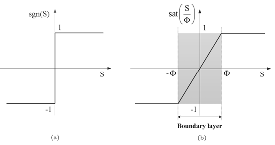
where \(k\) is a positive constant determining control strength, and \(\text{sgn}(S(x))\) is the signum function:

\[\text{sgn}(x) = \begin{cases} 1, & \text{if } x > 0 \\ 0, & \text{if } x = 0 \\ -1, & \text{if } x < 0 \end{cases} \tag{8}\]

The total control input thus becomes:

\[u = - \frac{f(x)}{g(x)} - k \text{sgn}(S(x)) \tag{9}\]

This control law ensures that the system state is driven to and maintained on the sliding surface, compensating for uncertainties and disturbances.

2. Advantages and Limitations

a) Advantages

• Exceptional robustness against model uncertainties and external disturbances
• Guaranteed finite-time convergence to the sliding surface
• Relatively simple implementation once the sliding surface is defined

b) Limitations

• Chattering: High-frequency switching of the control input can cause wear on actuators
• Model dependence: Extreme changes in system dynamics may require controller adjustments
• Design complexity: Requires deep understanding of system dynamics for optimal performance

3. Applications

SMC finds wide application in fields requiring robust control under dynamic conditions:

1. Robotics: Arm manipulation, mobile robot navigation
2. Automotive systems: Anti-lock braking, active suspension control
3. Aerospace engineering: Spacecraft attitude control, flight systems
4. Power systems: Converters, wind turbine control
5. Process control: Chemical reactors, temperature regulation
6. Biomedical systems: Prosthetic limb control, drug delivery

The versatility and robustness of SMC make it a valuable tool across various engineering disciplines, particularly where precise control is crucial despite uncertainties and disturbances.

II. Mathematical Modeling and Analysis

1. Implementing SMC for Inverted Pendulum

To apply Sliding Mode Control to our inverted pendulum system, we need to derive the system equations in a form suitable for SMC implementation. Let’s walk through this process step by step.

a) Deriving System Equations

1. Starting Point: Equation of Motion we begin with the equation of motion from our previous analysis:

   \[\begin{bmatrix} m_0 + m_1 & -\frac{1}{2}m_1 l_1 \cos\theta \\ -\frac{1}{2}m_1 l_1 \cos\theta & \frac{1}{3}l_1^2 m_1 \end{bmatrix} \begin{bmatrix} \ddot{x} \\ \ddot{\theta} \end{bmatrix} + \begin{bmatrix} \frac{1}{2}m_1 l_1 \sin\theta \cdot\dot{\theta}^2 \\ 0 \end{bmatrix} + \begin{bmatrix} 0 \\ - \frac{1}{2}g m_1 l_1\sin\theta \end{bmatrix} = \begin{bmatrix} F \\ 0 \end{bmatrix} \tag{10}\]

2. Solving for Accelerations To obtain expressions for \(\ddot{x}\) and \(\ddot{\theta}\), we invert the mass matrix:

   \[\begin{bmatrix} \ddot{x} \\ \ddot{\theta} \end{bmatrix} = \begin{bmatrix} m_0 + m_1 & -\frac{1}{2}m_1 l_1 \cos\theta \\ -\frac{1}{2}m_1 l_1 \cos\theta & \frac{1}{3}l_1^2 m_1 \end{bmatrix}^{-1} \begin{bmatrix} F - \frac{1}{2}m_1 l_1 \sin\theta \cdot\dot{\theta}^2\\ \frac{1}{2}g m_1 l_1\sin\theta \end{bmatrix} \tag{11}\]

3. Explicit Expressions After performing the matrix operations, we get:

   \[\begin{bmatrix} \ddot{x} \\ \ddot{\theta} \end{bmatrix} = \begin{bmatrix} \frac{4F - 2m_1l_1\sin\theta\cdot\dot{\theta}^2 + 3gm_1\cos\theta\sin\theta}{4m_0 + 4m_1 - 3m_1\cos^2\theta} \\ \frac{6\cos\theta(F - \frac{1}{2}m_1l_1\sin\theta\cdot\dot{\theta}^2)}{l_1(4m_0 + 4m_1 - 3m_1\cos^2\theta)} + \frac{6g(m_0 + m_1)\sin\theta}{l_1(4m_0 + 4m_1 - 3m_1\cos^2\theta)} \end{bmatrix} \tag{12}\]

4. SMC-Compatible Form For SMC implementation, we need to express our system’s equations of motion in a form that separates the system dynamics from the control input:

   \[\begin{aligned} \ddot{x} &= f_x(q, \dot{q}) + g_x(q)u \\ \ddot{\theta} &= f_{\theta}(q, \dot{q}) + g_{\theta}(q)u \end{aligned} \tag{13}\]

   where \(q = (x, \theta)^T\) represents the generalized coordinates, \(\dot{q} = (\dot{x}, \dot{\theta})^T\) are their derivatives, and \(u = F\) is our control input.

   This form separates the nonlinear dynamics (\(f_x\) and \(f_{\theta}\)) from the control influence (\(g_x\) and \(g_{\theta}\)), which is crucial for SMC design. Comparing with our explicit expressions in (11), we can identify:

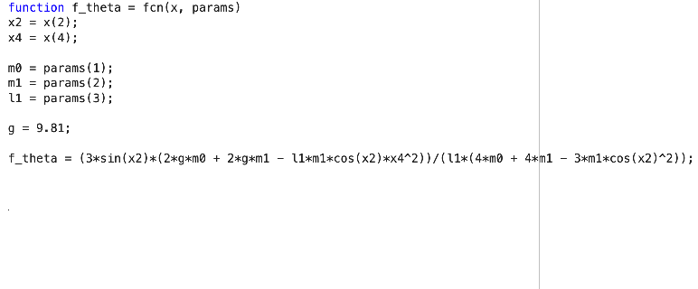
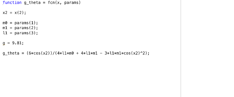
   \[f_x(q, \dot{q}) = \frac{m_1\sin\theta(3g\cos\theta - 2l_1\dot{\theta}^2)}{4m_0 + 4m_1 - 3m_1\cos^2\theta} \tag{14}\] \[g_x(q) = \frac{4}{4m_0 + 4m_1 - 3m_1\cos^2\theta} \tag{15}\] \[f_{\theta}(q, \dot{q}) = \frac{3\sin\theta(2gm_0 + 2gm_1 - l_1m_1\cos\theta\cdot\dot{\theta}^2)}{l_1(4m_0 + 4m_1 - 3m_1\cos^2\theta)} \tag{16}\] \[g_{\theta}(q) = \frac{6\cos\theta}{l_1(4m_0 + 4m_1 - 3m_1\cos^2\theta)} \tag{17}\]

These equations now provide us with the necessary structure to design our Sliding Mode Controller for the inverted pendulum system.

b) Sliding Mode Controller Design

In this section, we will implement the decoupled sliding mode control based on the work of Coban and Ata (2017): Decoupled sliding mode control of an inverted pendulum on a cart: An experimental study. This approach separates the control of the cart’s position and the pendulum’s angle, offering potentially better performance than coupled control methods.

Note: There is an alternative coupled sliding mode control approach by Park and Chwa (2009): Swing-Up and Stabilization Control of Inverted-Pendulum Systems via Coupled Sliding-Mode Control Method, which we plan to implement in future work.

1. Decoupled Sliding Surfaces

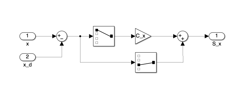
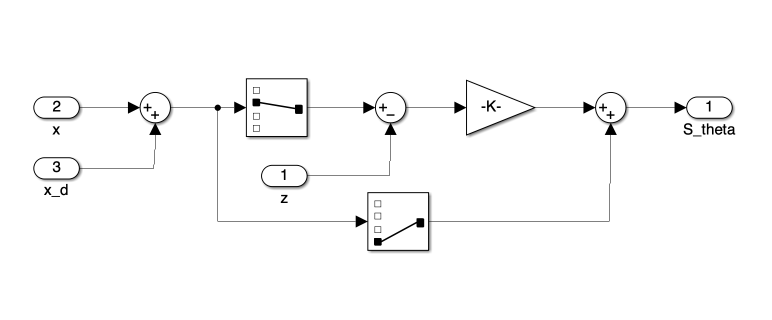
   we define two separate sliding surfaces, \(S_x\) for the cart position and \(S_{\theta}\) for the pendulum angle:

   \[S_{x} = C_x x +\dot{x} \tag{18}\] \[S_{\theta} = C_{\theta}\left(\theta - z\right) + \dot{\theta} \tag{19}\]

   where:

   • \(C_x\) and \(C_{\theta}\) are positive constants that determine the slope of the sliding surfaces
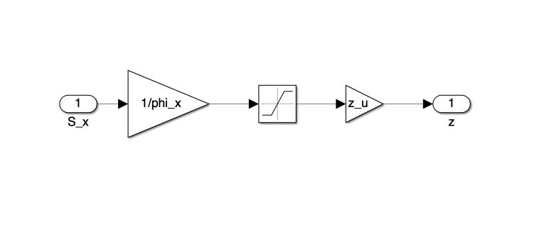
   • \(z\) is a nonlinear function that couples the two sliding surfaces:
   \[z = \text{sat}\left(\frac{S_x}{\phi_x}\right)z_u \tag{20}\]

   The saturation function \(\text{sat}\) is defined as:

   \[\text{sat}(\gamma) = \begin{cases} \text{sgn}(\gamma) & \text{for } |\gamma|\ge 1 \\ \gamma & \text{for } |\gamma| < 1 \end{cases} \tag{21}\]

   Here, \(0<z_u<1\) is a design parameter, and \(\phi_x\) is a positive constant.

2. Control Law

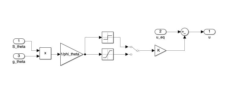
   The control law is designed as:

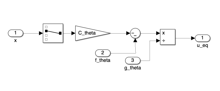
   \[u = u_{eq} - K\text{sat}\left(S_{\theta}\frac{g_{\theta}}{\phi_{\theta}}\right) \tag{22}\]

   where:

   • \(u_{eq}\) is the equivalent control term:
   \[u_{eq} = \frac{-C_{\theta}\theta-f_{\theta}}{g_{\theta}} \tag{23}\]
   • \(K\) is a positive constant gain
   • \(\phi_{\theta}\) is a positive constant similar to \(\phi_x\)
   • \(f_{\theta}\) and \(g_{\theta}\) are as defined in the previous section

This decoupled design allows for separate tuning of the cart position and pendulum angle control, potentially leading to improved overall system performance.

III. Simulink Implementation

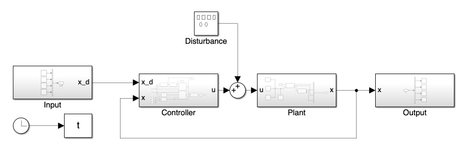
1. Overall System, Input/Output, and Plant

The fundamental structure of the overall system, including the input/output and plant blocks, remains consistent with the model presented in Day 6.

2. Controller Block

Figure 2 presents the block diagram of the SMC implementation. This diagram visually represents the interconnection of various components that make up our control system, each corresponding to specific equations derived in the previous section.

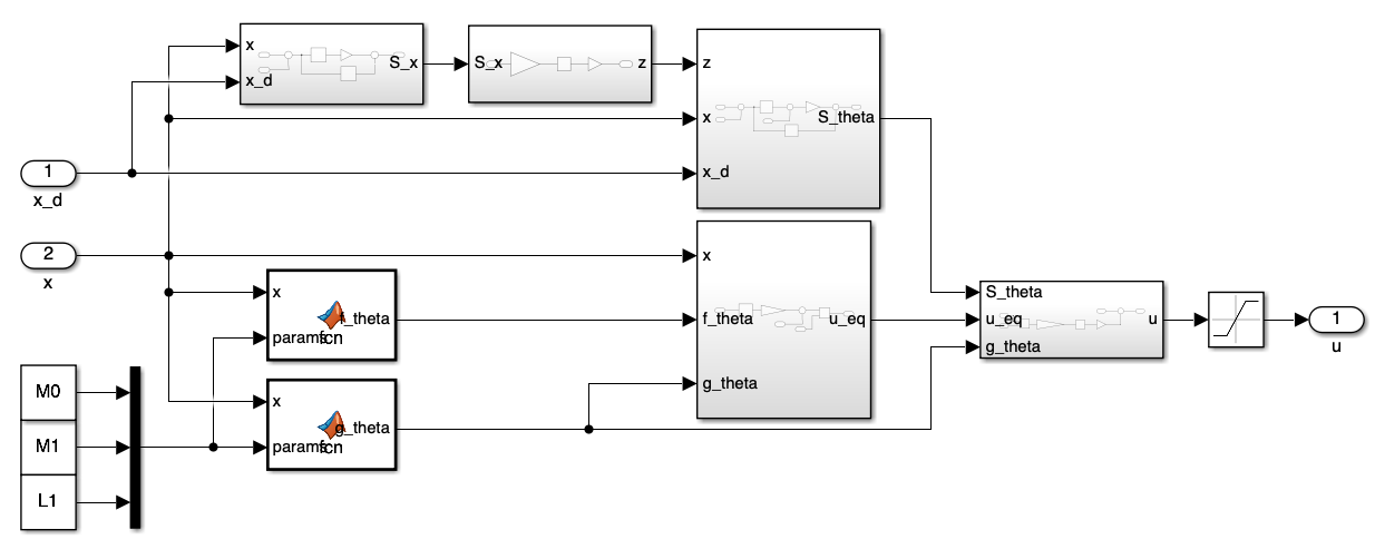
Each block in Figure 2 corresponds to Equations 16 through 23, which define the core elements of our SMC strategy. These individual components are further detailed in Figures 2 through 8, providing a closer look at their Simulink implementations.

Of particular note is the block representing Equation 22, shown in Figure 8. Here, we’ve incorporated both a saturation function (as per the decoupled SMC design) and a sign function, selectable via a manual switch. This modification allows for comparison between the proposed decoupled SMC and a more conventional SMC approach that uses a sign function instead of saturation.

IV. Simulation

1. Stability Test

To assess the system’s stability characteristics, we conducted a series of simulations with varying values of \(C_x\). The other system parameters were held constant as follows:

\[\begin{array}{l} C_{\theta} = 10, \quad \phi_x = 1, \quad \phi_{\theta} = 2.3 \\ K = 0.05, \quad z_u = 0.5, \quad d = 0 \end{array}\]

Where \(d\) represents the magnitude of disturbance, set to zero for this initial stability analysis.

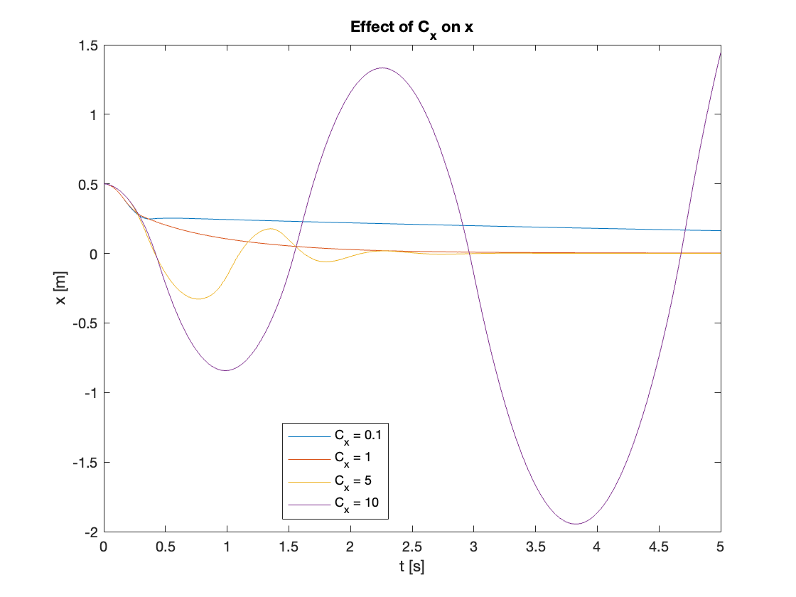
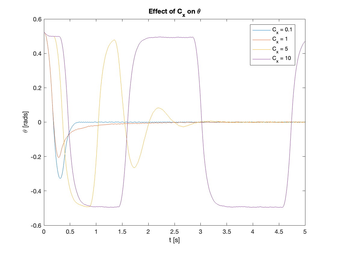
The key variable in this test was \(C_x\), which we varied across four values: [0.1, 1, 5, 10]. This range was chosen to observe the system’s behavior from very low to relatively high values of \(C_x\).

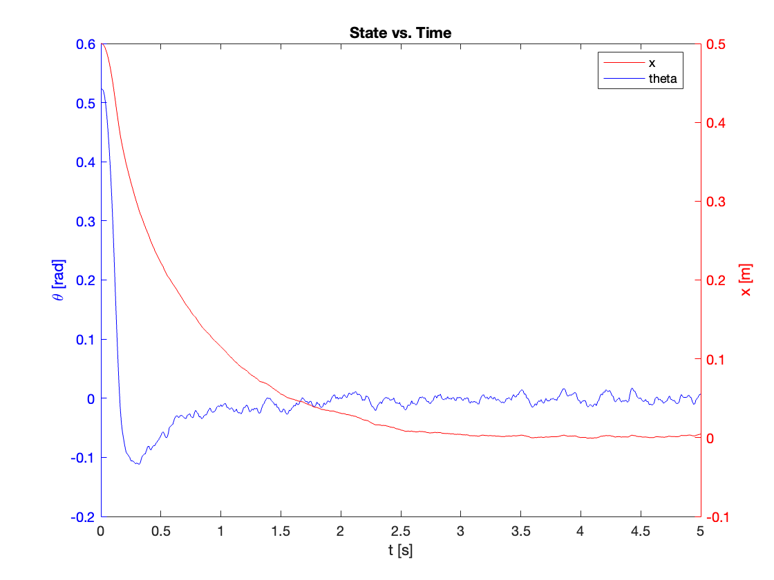
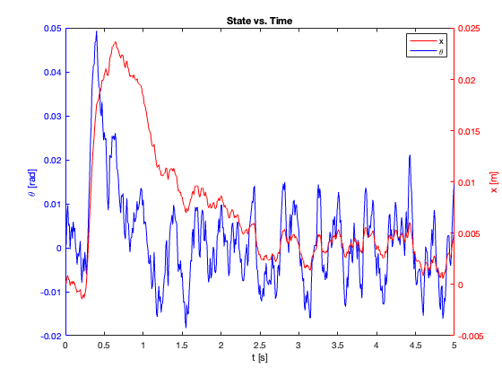
The results of these simulations, presented in Video 1 and Figures 10-15, reveal three distinct stability regimes as \(C_x\) increases:

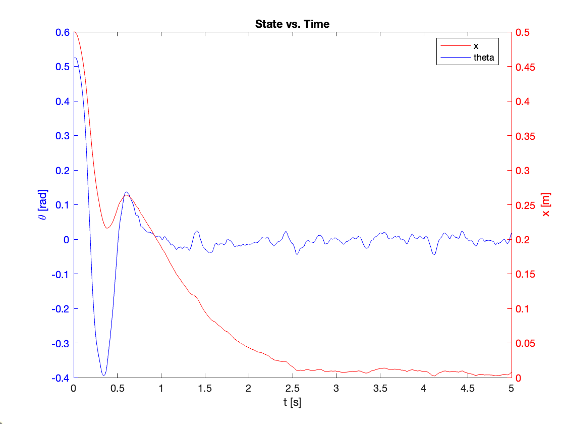
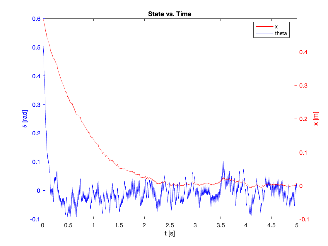
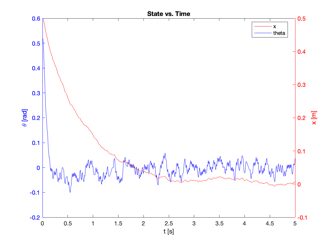
• Stable (\(C_x = 0.1, 1, 5\)):
  • Both \(x\) and \(\theta\) converge to equilibrium
  • As \(C_x\) increases:
    • Settling time (\(t_{ss}\)) initially decreases
    • System response transitions from overdamped to underdamped
  • At \(C_x = 5\), oscillations become more pronounced, indicating approach to stability limit

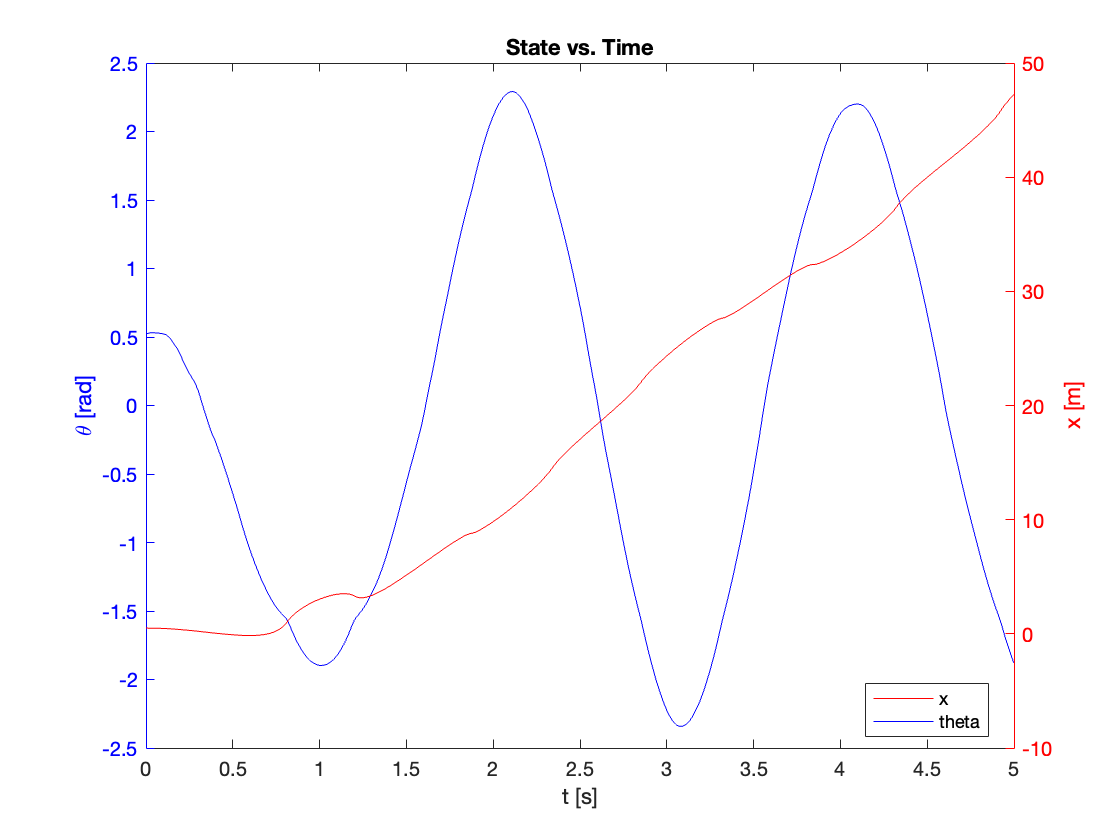
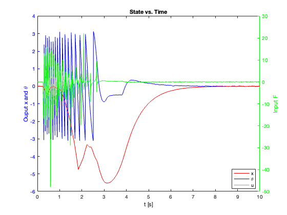
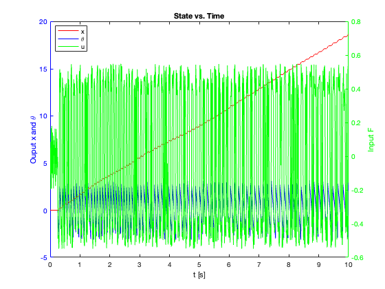
• Marginally Stable (\(\theta\) when \(C_x = 10\)):
  • \(\theta\) oscillates with constant amplitude of 0.5
  • Oscillation period increases over time

• Unstable (\(x\) when \(C_x = 10\)):
  • \(x\) diverges
  • Both amplitude and period of oscillations increase over time

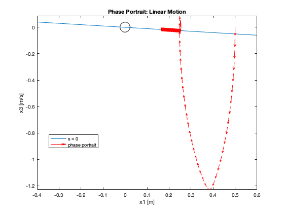
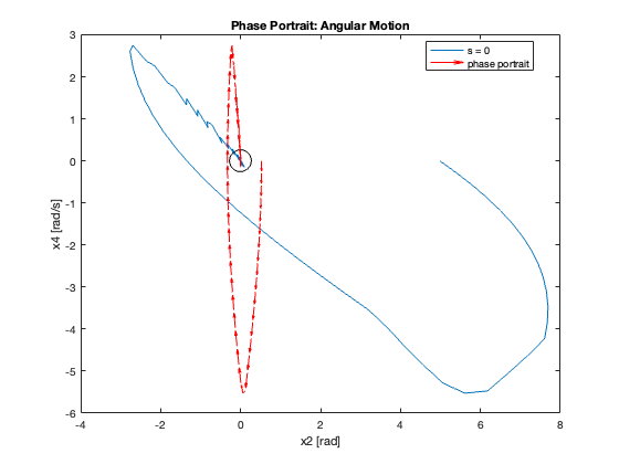
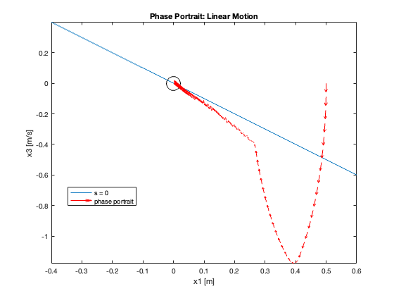
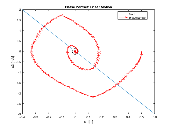
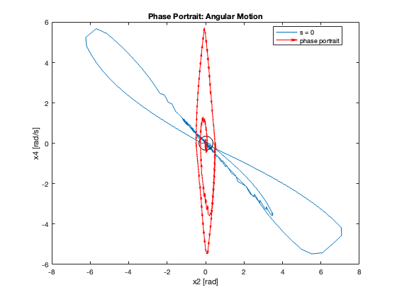
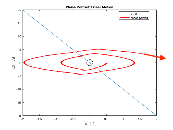
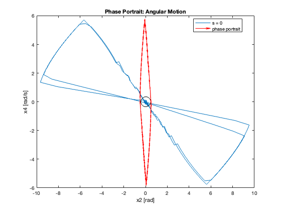
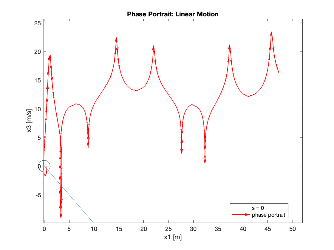
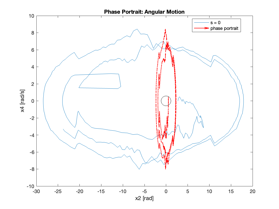
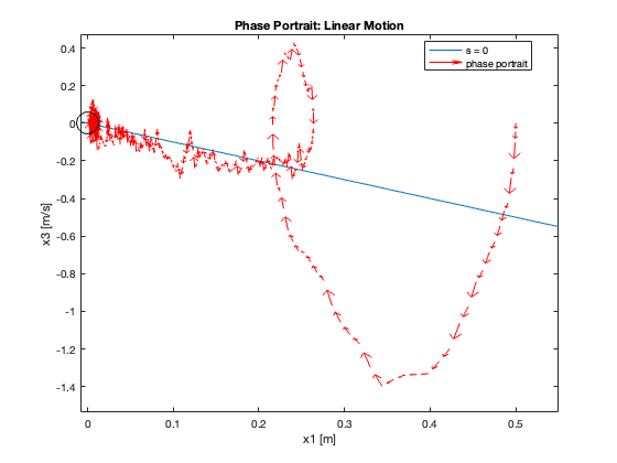
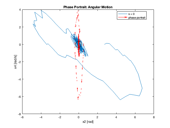
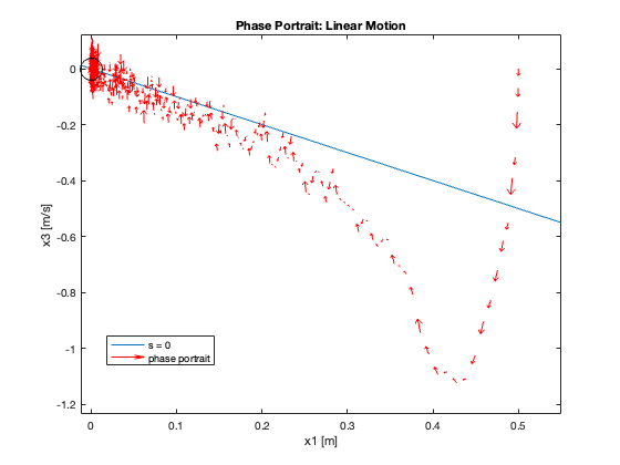
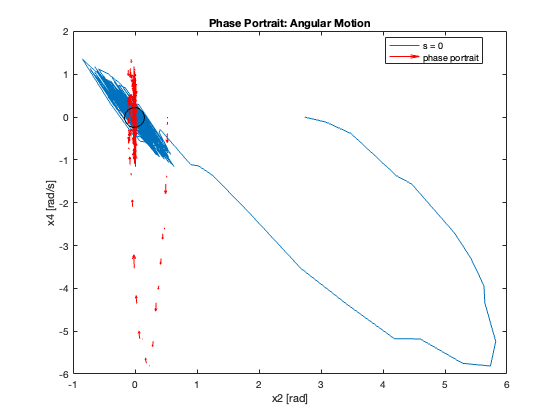
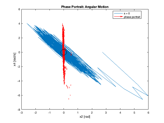
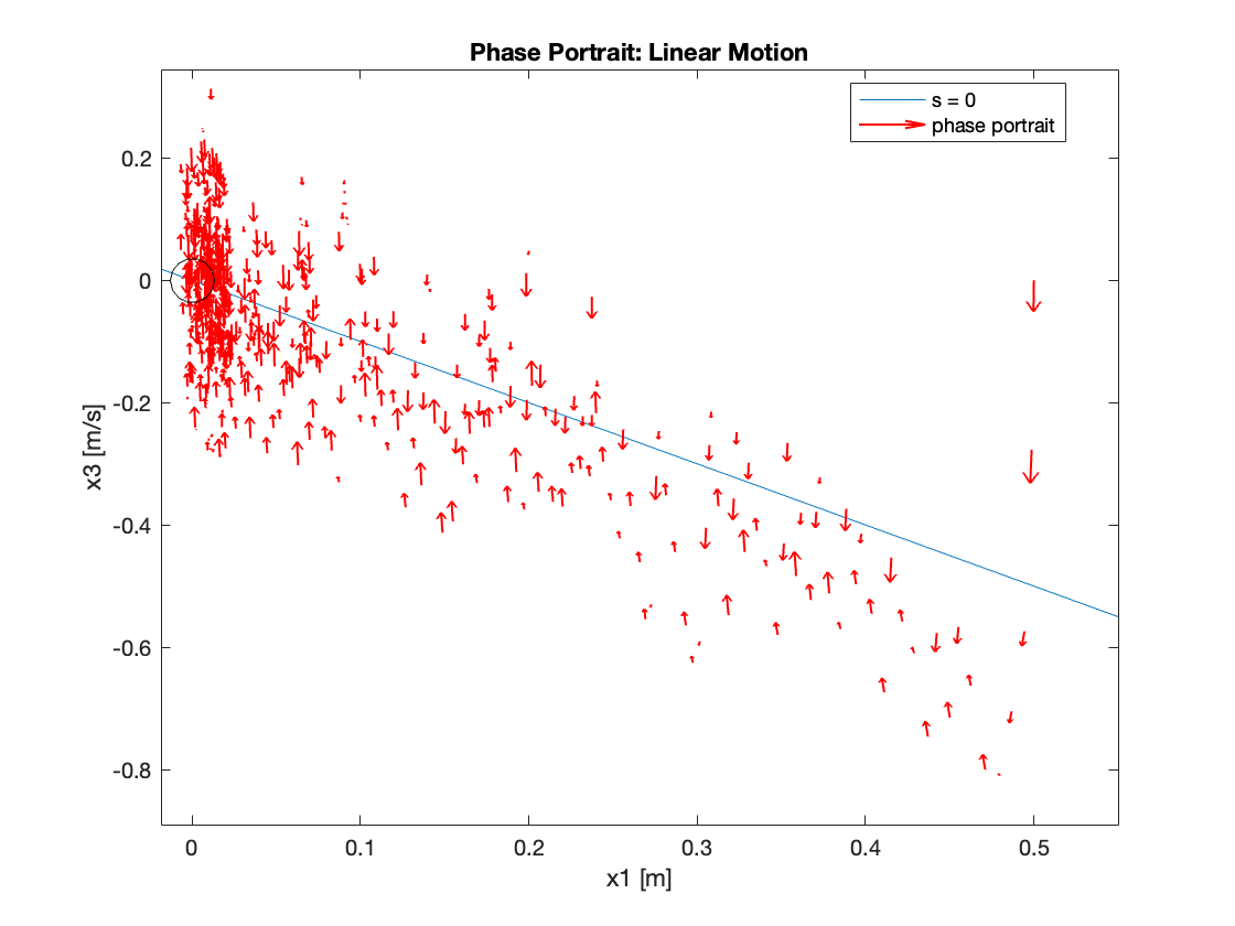
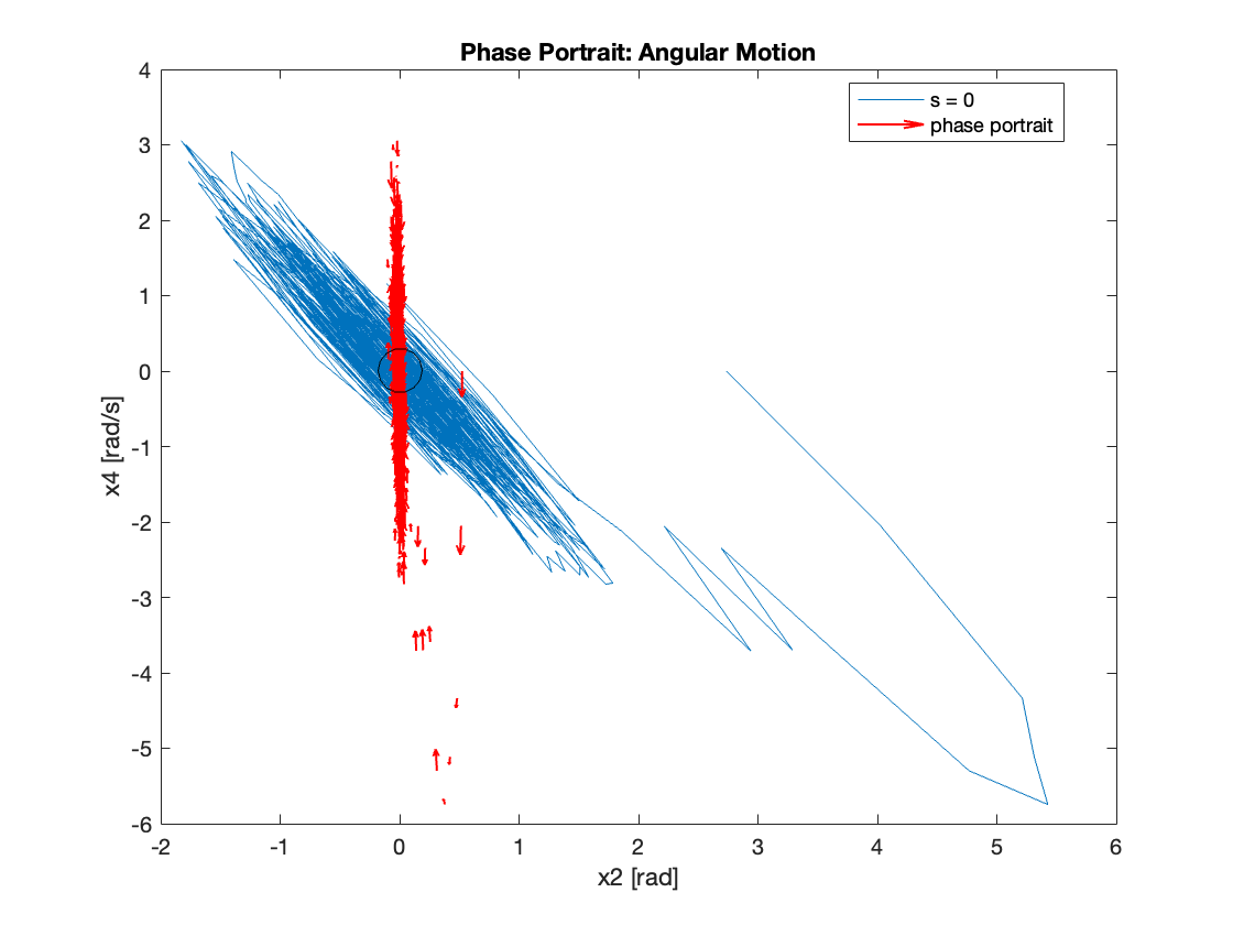
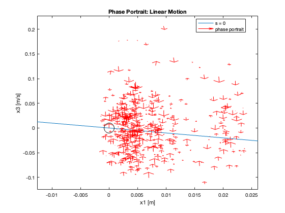
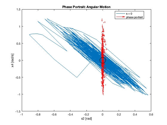
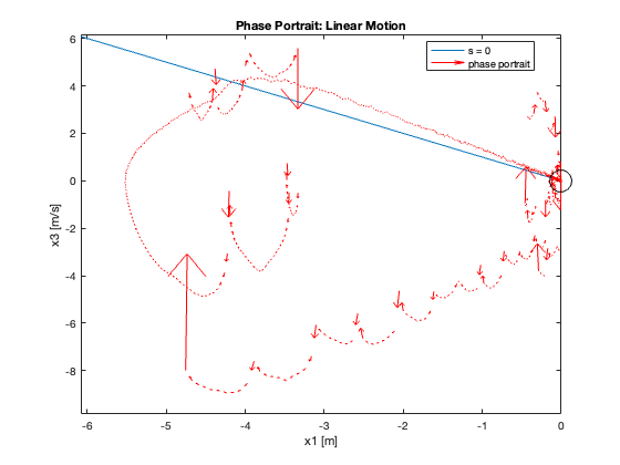
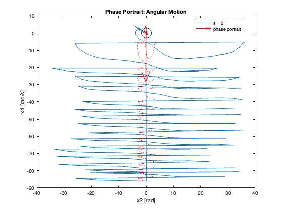
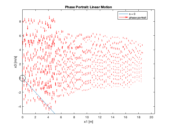
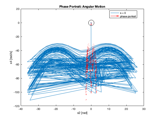
Phase Portrait Analysis:

• System trajectory shows two distinct phases: reaching and sliding
• After reaching the sliding surface, system converges along this surface to equilibrium
• \(S_x=0\) appears as a straight line (constant \(C_x\)), while \(S_{\theta}\) is nonlinear (due to \(z\))
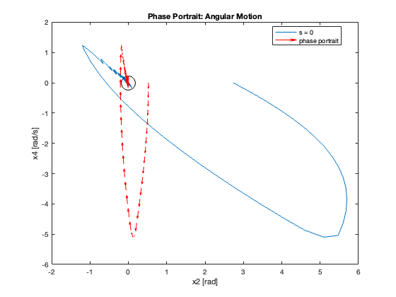
• For \(C_x = 10\), phase portrait shows \(x\) diverging and \(\theta\) in a limit cycle

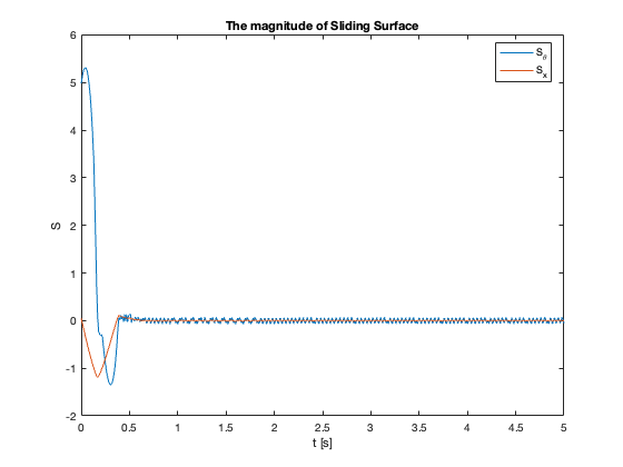
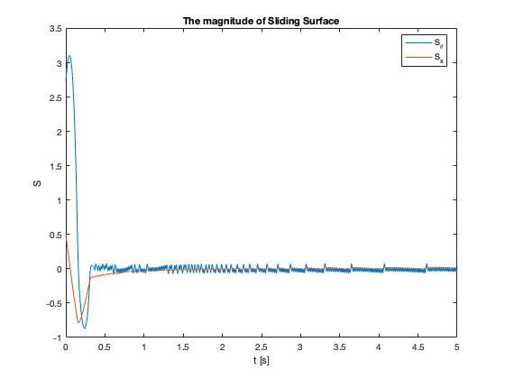
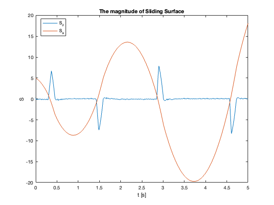
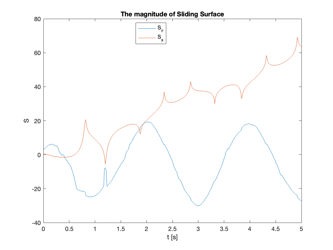
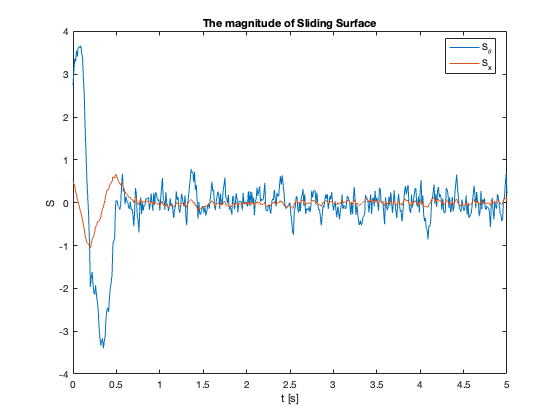
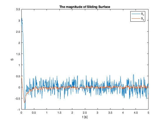
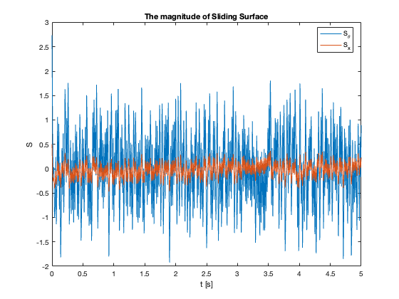
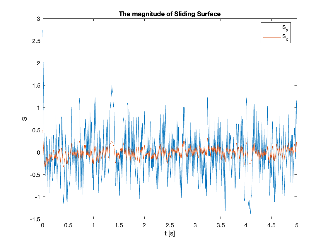
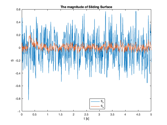
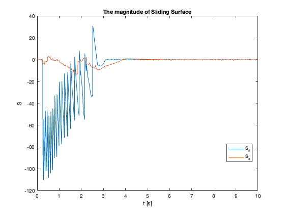
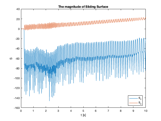
Sliding Surface Analysis: The behavior of the sliding surfaces \(S_x\) and \(S_{\theta}\) provides valuable insights into the system’s dynamics across different \(C_x\) values:

• \(C_x = 1\) compared to \(C_x = 0.1\):
  • \(S_{\theta}\) reaches zero faster
  • \(S_x\) reaches zero slower
  • Key Insight: Faster convergence to sliding surfaces doesn’t necessarily mean faster overall stabilization
  • Observation: Reaching mode may be faster while Sliding mode is slower

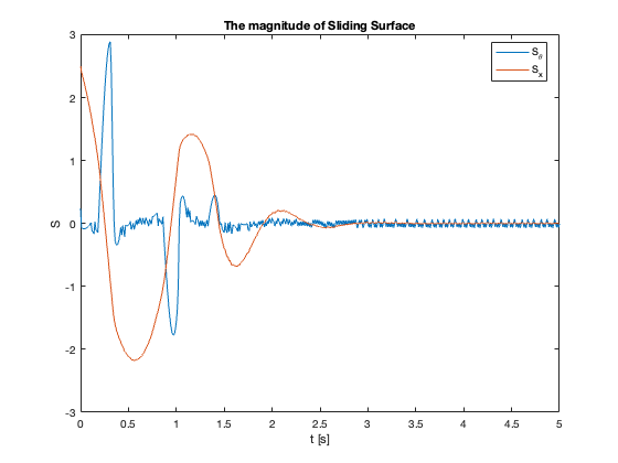
• \(C_x = 5\) :
  • Both \(S_x\) and \(S_{\theta}\) exhibit oscillations
  • Indicates approach to stability limit

• \(C_x =10\):
  • \(S_{\theta}\) remains mostly at zero
  • \(S_x\) diverges
  • Despite \(S_{\theta}=0\), \(\theta \neq 0\) (not at equilibrium)
  • Key Insight: \(S = 0\) does not imply the system is at equilibrium but in Sliding Mode

General Observations:

1. The relationship between sliding surface convergence and system stabilization is not always straightforward.
2. Oscillations in sliding surfaces can indicate impending instability.
3. Achieving \(S=0\) is necessary but not sufficient for system equilibrium, especially at higher \(C_x\) values.

In summary, as \(C_x\) increases, we observe a transition from slow, overdamped response to faster response with oscillations, eventually leading to instability. This progression highlights the critical trade-off between convergence speed and stability in the system’s design.

2. Effect of Switching Term Gain (\(K\))

This section examines the impact of the switching term gain (\(K\)) in the control input:

\[u = u_{eq} - K\text{sat}\left(S_{\theta}\frac{g_{\theta}}{\phi_{\theta}}\right) \tag{22}\]

Parameters were set as follows:

\[\begin{array}{l} C_x = 1, \quad C_{\theta} = 10, \quad \phi_x = 1 \\ \phi_{\theta} = 2.3, \quad z_u = 0.5, \quad d = 0.1 \end{array}\]

we varied \(K\) across [0.01, 0.05, 0.1, 1]. The results are shown in Video 2 and Figures 16-19.

Key Observations:

• Low \(K=0.01\):
  • Insufficient resistance against disturbances
  • System becomes unstable

• Moderate \(K = 0.05, 0.1\):
  • Improved stability
  • Faster reaching mode as K increases
• High \(K=1\):
  • Very quick reaching of sliding surface
  • Significant chattering observed
  • Potential instability due to excessive chattering

General Findings:

• As K increases, the speed of reaching mode improves
• Higher K values lead to increased chattering due to overreaction
• Extreme chattering can cause system instability

The Figures (b) clearly illustrate these effects, particularly the increased chattering at higher K values.

3. Mitigating Chattering Effects

To address the chattering observed in our initial simulations, two potential solutions were identified:

1. Adaptive Gain: Vary \(K\) based on the distance between states and the sliding surface.
2. Alternative Functions: Replace \(\text{sgn}(x)\) with a continuous function to reduce chattering effects.

Implementation of Saturation Function

To test the second approach, we replaced \(\text{sgn}(x)\) with \(\text{sat}(x)\), maintaining \(K=1\). The results are shown in Figure 20.

Key Observations:

1. Reduced Chattering: The average magnitude of chattering decreased from 1 to 0.5.
2. Similar Disturbance Resistance: The system showed comparable resistance to disturbances as the original \(\text{sgn}(x)\) function, which is expected since \(K\) remained the same.

4. Regulation

After examining tracking performance in Sections 1-3, this section focuses on the system’s regulation capabilities under external forces.

\[\begin{array}{l} C_x = 1, \quad C_{\theta} = 10, \quad K = 0.1 \\ \phi_x = 1, \quad \phi_{\theta} = 2.3, \quad z_u = 0.5, \quad d = 0.1 \end{array}\]

The controller employed the \(\text{sgn}(x)\) function, and external forces of \(F = [0.2, 0.5]\) were applied to test regulation performance.

The regulation performance is illustrated in Video 3 and Figures 21-22.

Key Observations:

1. Robust Performance: The controller demonstrated good regulation capabilities for both external force magnitudes.
2. Disturbance Rejection: The system successfully maintained stability and returned to equilibrium despite the applied forces.

5. Extreme Cases

This section examines the controller’s robustness under extreme conditions, specifically swing-up motion and high external forces. These tests reveal important insights into the controller’s limitations and the impact of input saturation.

Methodology

• Tested two scenarios: swing-up motion (tracking) and high external force (regulation)
• Compared performance with and without input saturation
• Saturation limit set to 0.45, consistent with previous posts

Key Findings

• Without Saturation:
  • The system consistently converged to the equilibrium point
  • Robust performance regardless of initial state or external force magnitude

• With Saturation (0.45):
  • Controller performance significantly degraded
  • In most cases, the system became unstable
  • Notably, this SMC showed instability where other controllers remained stable under the same conditions

23-24: Tracking performance during swing-up motion (without and with saturation)
25-26: Regulation performance under high external force (without and with saturation)

V. Conclusion

In this study, we implemented a Sliding Mode Control (SMC) strategy for an inverted pendulum system, incorporating both stabilization and swing-up control. This approach demonstrated significant potential in managing the nonlinear dynamics of the inverted pendulum, offering insights into robust control for complex mechanical systems.

Key findings from our simulations include:

1. The SMC effectively managed both swing-up and stabilization tasks in the absence of input saturation, demonstrating robustness against small to moderate disturbances and parameter variations.

2. The controller’s performance was highly sensitive to parameter choices, highlighting the critical importance of careful tuning.

3. Replacing the sign function with a saturation function in the control law successfully mitigated chattering, a common issue in SMC implementations, without compromising performance.

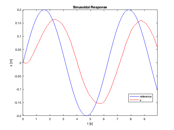
4. While excelling in stabilization, the SMC showed limitations in tracking performance, especially for rapidly changing reference signals, as illustrated in Figure 27.

However, our work also revealed areas for further improvement:

1. Enhancing robustness under extreme conditions and input saturation.

2. Developing adaptive strategies to handle extreme initial states and large disturbances.

3. Integrating SMC with complementary techniques (e.g., energy shaping) for a more robust swing-up strategy under input saturation constraints.

These research directions promise to push the boundaries of nonlinear control systems, bringing us closer to robust, generalizable solutions for complex mechanical systems. Stay tuned for future updates as we continue to explore and innovate in the fascinating realm of advanced control strategies!

You can find the Simulink model on my GitHub repository.

\[\]