I. Overview and Contributions

1. Paper Overview

This paper addresses critical challenges in the control of Series Elastic Actuators (SEAs) within cascaded control architectures, which include both impedance and torque feedback loops. It proposes a comprehensive framework for optimizing SEA performance, particularly focusing on impedance control while accounting for real-world factors such as time delays and filtering. The authors introduce a critically damped gain design criterion that enhances system stability and performance by optimizing controller gains based on phase-margin-based stability. A key contribution is the concept of the “Z-region,” a novel metric that quantifies the achievable impedance magnitude and frequency ranges, providing a unified characterization of SEA performance. The validity of the proposed methods is demonstrated through simulations and experiments.

2. Challenges and Gaps in Previous Research

Previous SEA control and performance optimization research faced several limitations:

• Existing methods often relied on empirical tuning or provided undetermined gains.
• Characterization of SEA impedance performance, considering both magnitude and frequency ranges, was inadequate.
• Effects of time delays, filtering, and load inertia on SEA impedance were not thoroughly analyzed.
• Most literature focused on low SEA impedance for compliant control, limiting capabilities for stiff tasks.

3. Key Contributions and Advancements

To address these limitations, the paper offers several significant advancements:

1. A critically damped gain design method for SEA cascaded control architectures.
2. Analysis of the tradeoff between impedance and torque controller gains.
3. Frequency-domain methods to analyze effects of time delays, filtering, and load inertia on SEA impedance.
4. The “Z-region” metric, quantifying both achievable impedance magnitude (Z-width) and frequency ranges (Z-depth).

II. Technical Analysis and Methodology

1. SEA Controller Diagram

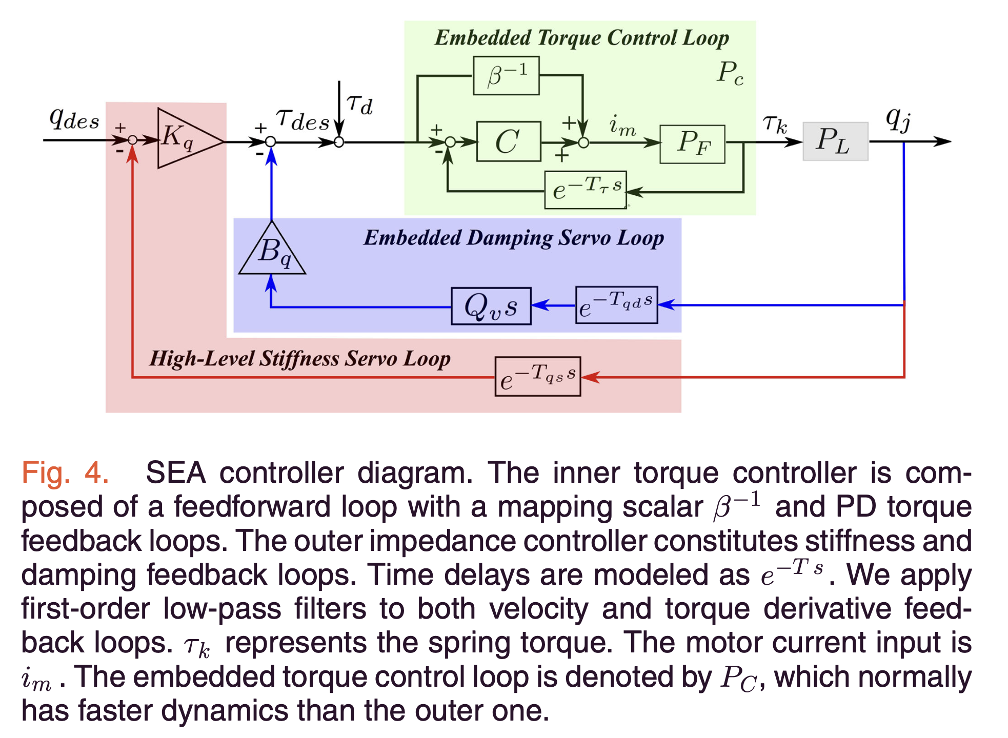
The SEA controller diagram (Figure 4) illustrates a cascaded control architecture with two main feedback loops:

1. Torque Control Loop (\(P_C\)) The inner torque control loop \(P_C(s)\) ensures precise torque tracking in SEAs. It comprises:
   • A feedforward component mapping desired torque to motor current
   • A Proportional-Derivative (PD) feedback controller
   • A first-order low-pass filter for noise management

   The transfer function for this loop is:

   \[P_C(s) = \frac{\tau_k(s)}{\tau_{\text{des}}(s)} = \frac{P_F (\beta^{-1} + C)}{1 + P_F C e^{-T_\tau s}}\]

   Where \(P_F(s)\) is the SEA plant model, \(C = K_\tau + B_\tau Q_{\tau d}s\) is the PD compensator, \(Q_{\tau d}\) is the first-order low-pass filter, and \(e^{-T_\tau s}\) represents the delay term.

2. Impedance Feedback (\(\tau_{des}\)) This loop generates the desired torque \(\tau_{des}\) based on position errors and their derivatives. It includes:
   • Stiffness (\(K_q\)) and damping (\(B_q\)) feedback loops
   • Associated time delays for each feedback path

   The impedance feedback is described by:

   \[\tau_{des}(s) = K_q (q_{des} - e^{-T_{qs} s} sq_j) - B_q e^{-T_{qd} s} Q_{qd} sq_j\]

   Where \(q_{des}\) is the desired joint position, \(e^{-T_{qs} s}\) and \(e^{-T_{qd} s}\) are time delays, and \(Q_{qd}\) is the velocity filter.

3. SEA Closed-Loop Transfer Function (\(P_{CL}\))

   This function captures the overall closed-loop behavior of the SEA system:

   \[P_{CL}(s) = \frac{q_j(s)}{q_{\text{des}} (s)} = \frac{K_q P_C P_L}{1 + P_C P_L (e^{-T_{qd} s} B_q Q_{qd} s + e^{-T_q s} s K_q)}\]

   Here, \(P_L(s)\) represents the load plant model (joint dynamics), and \(P_C(s)\) is the torque control loop transfer function.

2. Gain Design

a) Critically Damped Controller Gain Design Criterion

The authors propose a structured, analytically-based approach to designing controller gains, ensuring critical damping of the SEA system. This criterion involves the following key aspects:

1. Fourth-Order System Approximation: The complex SEA system, with its cascaded impedance and torque feedback loops, is modeled as a fourth-order system. To simplify analysis, this system is approximated as two second-order systems in series:

   \[(s^2 + 2\zeta_1 \omega_1 s + \omega_1^2)(s^2 + 2\zeta_2 \omega_2 s + \omega_2^2)\]
2. Critical Damping Assumption: The method assumes critical damping by setting:
   • Damping ratios: \(\zeta_1 = \zeta_2 = 1\)
   • Natural frequencies: \(\omega_1 = \omega_2 \triangleq \omega_n = 2\pi f_n\)

   This simplification allows for a structured gain design process.

3. Gain Design Equations: Based on these assumptions, a set of nonlinear equations is derived:

   \[\frac{I_j b_m + I_m b_j + I_j \beta B_\tau k}{I_m I_j} = 4\omega_n\] \[\frac{k(I_j (1 + \beta K_\tau) + I_m + \beta B_\tau (b_j + B_q)) + b_j b_m}{I_m I_j} = 6\omega_n^2\] \[\frac{k(b_j + B_q)(1 + \beta K_\tau) + k(b_m + \beta B_\tau K_q)}{I_m I_j} = 4\omega_n^3\] \[\frac{(1 + \beta K_\tau)k K_q}{I_m I_j} = \omega_n^4\]

   These equations form a system of simultaneous nonlinear equations. By solving this system, we can determine the gains for both the torque (\(K_\tau, B_\tau\)) and impedance (\(K_q, B_q\)) controllers.

4. Uniform Gain Determination: A key advantage of this method is that by selecting a single natural frequency \(f_n\), all controller gains are uniformly determined. This significantly simplifies the gain tuning process, avoiding the need for complex, heuristic tuning procedures.

b) Tradeoff Between Torque and Impedance Control

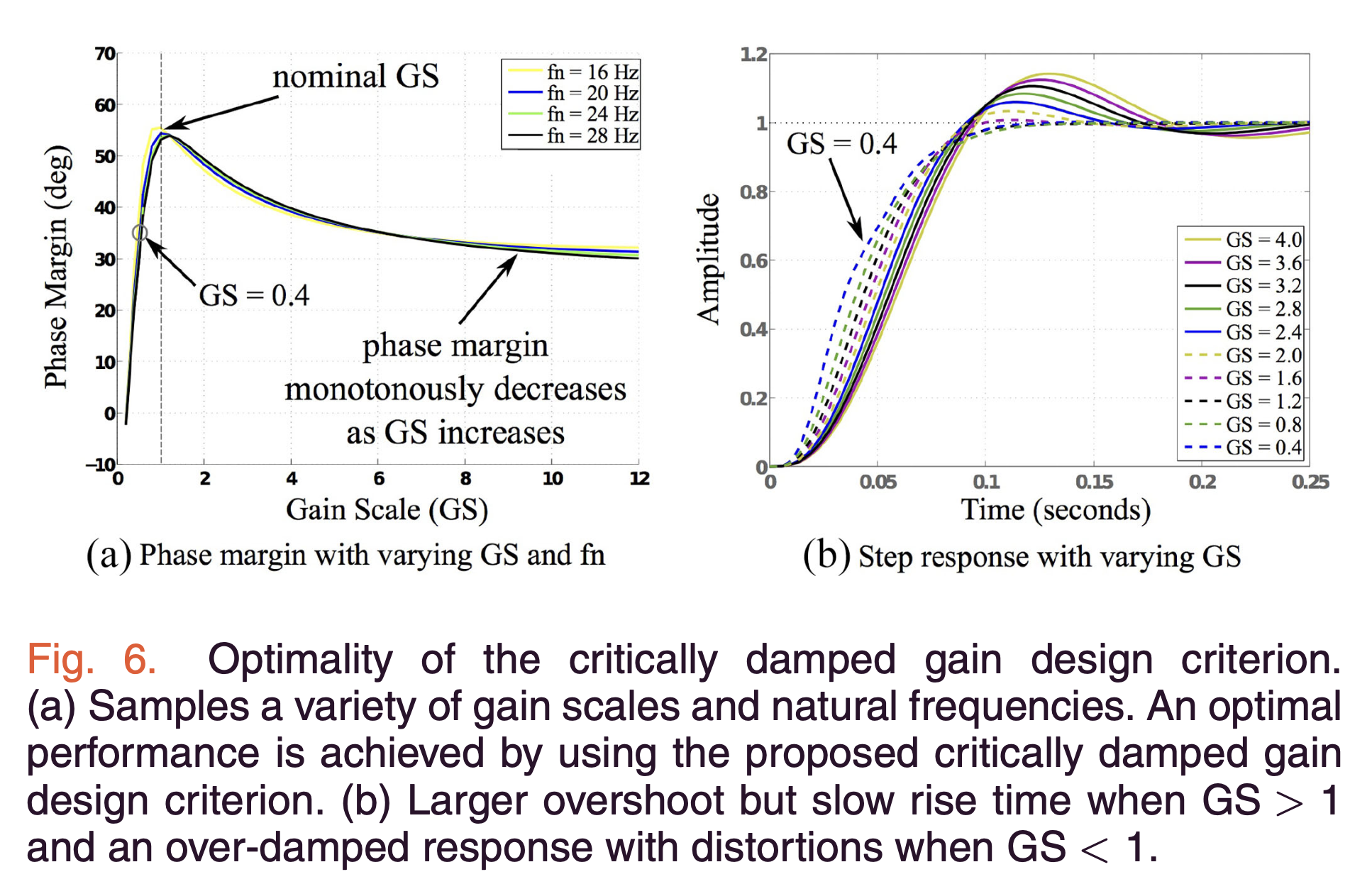
The authors identify and analyze a crucial tradeoff between torque and impedance control in SEAs, which impacts system stability. This analysis introduces the concept of Gain Scale and examines its effects on system performance:

1. Gain Scale Definition: The SEA Gain Scale (GS) is introduced as a parameter that scales torque and impedance gains relative to their nominal values:

   \[GS = \frac{K_{\tau a}}{K_{\tau n}} = \frac{K_{qn}}{K_{qa}}, \quad GS = \frac{B_{\tau a}}{B_{\tau n}} = \frac{B_{qn}}{B_{qa}}\]

   Where subscript \(a\) denotes adjusted gains and \(n\) denotes nominal gains designed by the critically damped criterion. A larger GS indicates increased torque gains with decreased impedance gains.

2. Impact on System Stability: Adjusting GS affects the system’s phase margin and response characteristics:
   • GS > 1: Higher torque gains and lower impedance gains lead to decreased phase margin and increased oscillations.
   • GS < 1: Lower torque gains and higher impedance gains result in an overdamped response with potential distortions.

3. Optimal Stability Point: The analysis confirms that GS = 1 (using gains from the critically damped criterion) achieves the best phase margin, ensuring optimal stability.

4. Performance Tuning: While GS = 1 offers optimal stability, varying GS allows for adjustments in impedance behavior, which can be beneficial for different applications.

3. Impedance Analysis

a) SEA Impedance Transfer Function

The authors derive a comprehensive SEA impedance transfer function:

\[Z(s) = \frac{\tau_j(s)}{-s q_j(s)} = \frac{\sum_{i=0}^{4} N_{zi} s^i}{\sum_{i=0}^{5} D_{zi} s^i}\]

Where:

• \(Z(s)\) is defined with a joint velocity \(\dot{q}_j\) input and a joint torque \(\tau_j\) output.
• This formulation is based on zero desired joint position \(q_{des}\).
• Numerator \(N_{zi}\) and denominator \(D_{zi}\) coefficients depend on system parameters, feedback gains, and time delay/filter parameters.
• This function explicitly models time delays and filtering effects, often neglected in traditional SEA models.

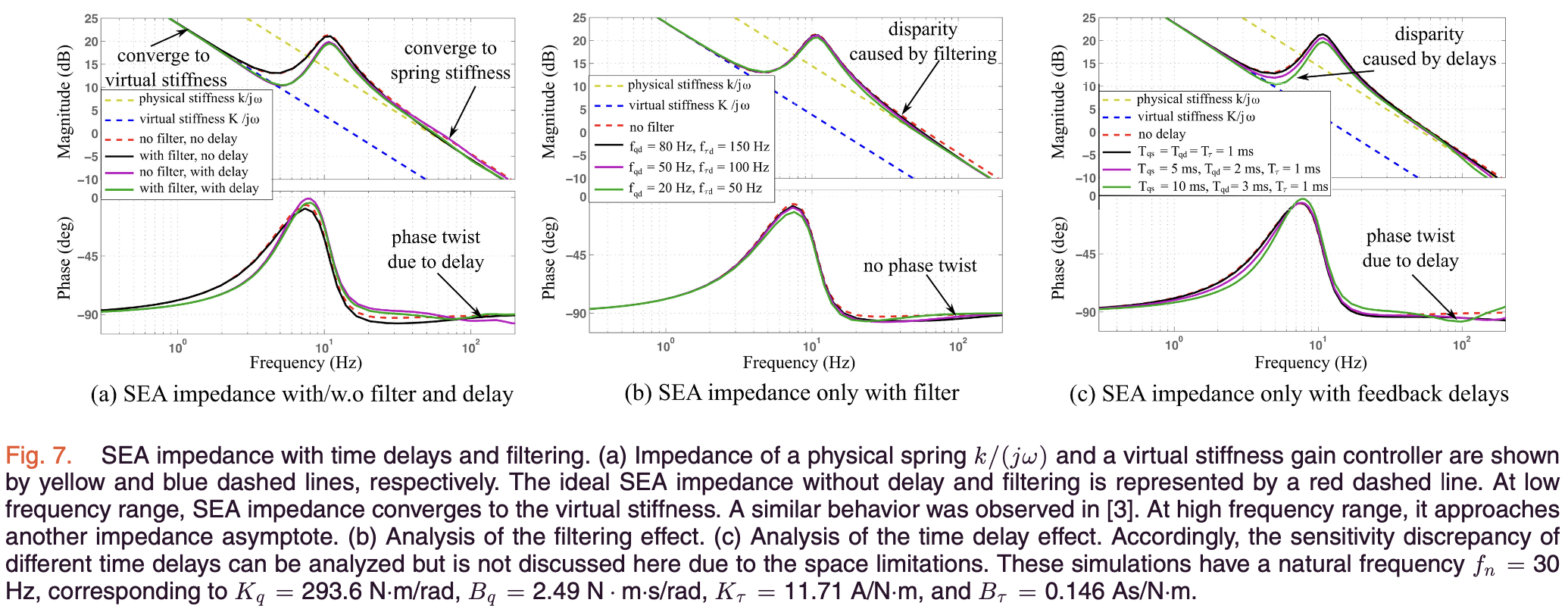
b) Effects of Time Delays and Filtering

The authors conduct a comprehensive analysis of how time delays and filtering impact SEA impedance behavior across different frequency ranges. This analysis reveals:

1. Scenario Analysis: Four scenarios are examined to isolate the effects of delays and filtering:

   • \(Z_i(j\omega)\): Ideal impedance (no delays or filtering)
   • \(Z_f(j\omega)\): Impedance with filtering only
   • \(Z_d(j\omega)\): Impedance with delays only
   • \(Z_{fd}(j\omega)\): Impedance with both delays and filtering

2. Low-Frequency Behavior: In all scenarios, the SEA impedance converges to a virtual stiffness asymptote:

   \[\lim_{\omega \to 0} Z_c(j\omega) = \frac{K_q k_\tau (\beta^{-1} + K_\tau)}{j\omega \cdot (1 + K_\tau k_\tau)}\]

   Where \(c \in \{i, f, d, fd\}\), representing the different scenarios.

3. High-Frequency Behavior: The impact of delays and filtering is most pronounced at high frequencies:

   • Ideal case: Approaches a constant stiffness-type impedance
   • With filtering: Converges to the passive spring stiffness without twisting
   • With delays: Shows periodic twisting around the passive spring stiffness
   • With both: Primarily exhibits twisting due to delays

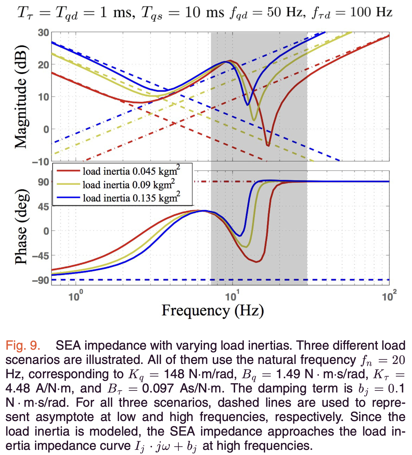
c) Effect of Load Inertia

The authors investigate how load inertia (\(I_j\)) influences SEA impedance characteristics, particularly at high frequencies. This analysis reveals:

1. Modified Impedance Model: The authors incorporate load inertia into the SEA impedance transfer function:

   \[Z_l(j\omega) = Z(j\omega) + I_j s + b_j\]

   Where \(Z(j\omega)\) is the original SEA impedance, \(I_j\) is the load inertia, and \(b_j\) is the damping coefficient.

2. Frequency-Dependent Behavior:

   • At high frequencies, the SEA impedance becomes dominated by load inertia:

     \[\lim_{\omega \to +\infty} Z_l(j\omega) = I_j \cdot j\omega + b_j\]

     This results in a 20 dB/decade increase in impedance magnitude.

   • In the mid-frequency range, filtering and time delays dominate, causing resonant spikes, while larger load inertia leads to smaller resonant spikes in the response

4. SEA Impedance Characterization

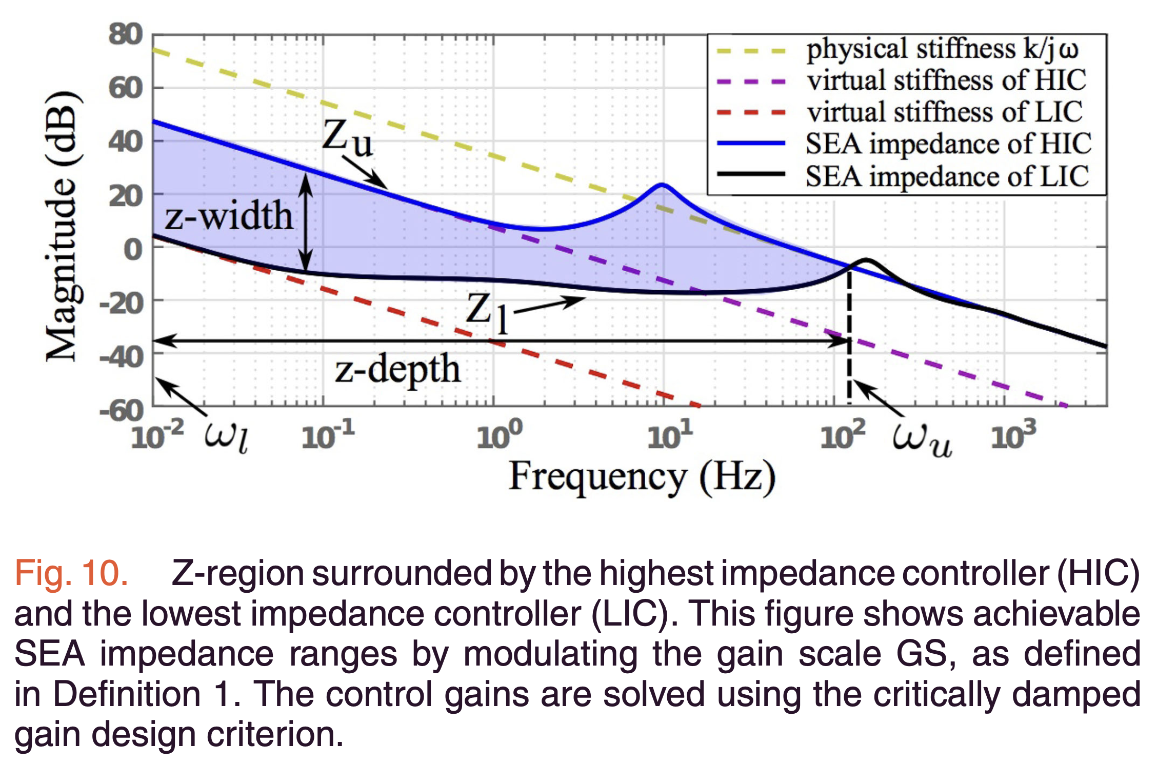
The authors introduce a novel metric, the “Z-region,” to comprehensively characterize SEA impedance performance. This metric quantifies both the achievable impedance magnitude range (Z-width) and the frequency range (Z-depth) of effective SEA operation.

a) Z-Region Definition

The Z-region is defined as the frequency-domain area where stable impedance control is achievable:

\[Z_{region} = \int_{\omega_l}^{\omega_u} W(\omega) \left| \log |Z_u(j\omega)| - \log |Z_l(j\omega)| \right| d\omega\]

Where:

• \(\omega_l\) and \(\omega_u\) are the lower and upper frequency boundaries
• \(Z_u\) and \(Z_l\) are the upper and lower impedance bounds
• \(W(\omega)\) is a frequency-dependent weighting function

b) Visualization and Analysis

The Z-region is visualized in Figure 10 as a blue shaded area:

• Bounded by the highest impedance controller (HIC) and lowest impedance controller (LIC)
• Demonstrates the trade-off between achievable impedance magnitude and frequency range

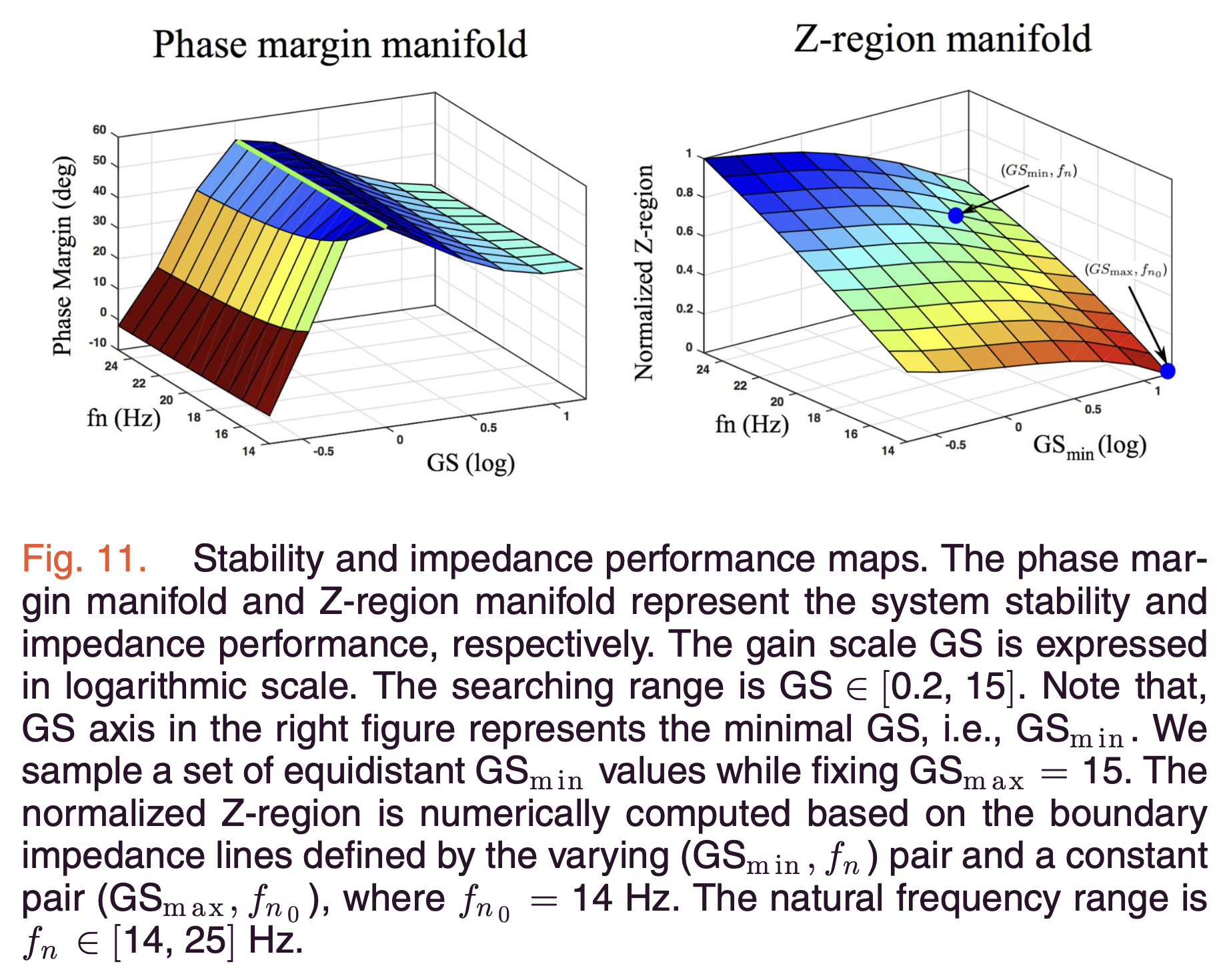
c) Performance Optimization

The authors demonstrate how adjusting the gain scale (GS) can optimize SEA performance within the Z-region:

• Figure 11 presents two key manifolds:
  1. System stability (phase margin)
  2. Impedance performance (Z-region)
• These manifolds are analyzed across various gain scales and natural frequencies

III. Personal Comments

The authors’ systematic approach to SEA control is impressive, particularly the critically damped gain design method which addresses the challenge of tuning cascaded control loops. The Z-region concept is innovative, offering a comprehensive measure of SEA performance that could be valuable for tasks requiring varied impedances across different frequency ranges.

However, the paper’s focus on linear models and controllers may limit its immediate applicability in real-world scenarios where nonlinear effects like friction and backlash are significant. Future work could extend these methods to account for such nonlinearities.

While the experimental validation is thorough, testing these methods on a full humanoid robot or in dynamic tasks like running or object manipulation would provide valuable insights into their practical limitations and potential.