Leadscrews are fundamental components in many mechanical systems, playing a crucial role in converting rotational motion into linear motion. From precision instruments to heavy machinery, leadscrews are ubiquitous in fields ranging from manufacturing to robotics. Understanding the dynamics of leadscrew systems is essential for engineers and designers aiming to optimize performance, improve efficiency, and enhance control in various applications.

In this post, we’ll examine the mathematical modeling of leadscrew systems. By deriving the equations of motion, we’ll gain insights into how various factors influence the behavior of these systems. This understanding is crucial for predicting system response, designing control systems, and improving overall performance.

I. Key Parameters

Before delving into the equations, let’s define the key parameters in our leadscrew system:

Parameter	Definition	Explanation	Unit
\(J\)	Moment of inertia of the screw	The screw’s resistance to rotational acceleration	\(kg\, m^2\)
\(B_r\)	Rotational damping coefficient	Energy losses in rotational motion	\(N \, m \, s/rad\)
\(\theta\)	Angular displacement of the screw	The screw’s rotation angle	\(rad\)
\(T\)	Applied torque to the screw	The rotational force driving the system	\(N \, m\)
\(T_{\text{friction}}\)	Frictional torque	Torque opposing motion due to friction	\(N \, m\)
\(m\)	Mass of the load	The weight moved by the leadscrew	\(kg\)
\(b_t\)	Translational damping coefficient	Energy losses in linear motion	\(N \, s/m\)
\(k\)	Stiffness of the system	The system’s resistance to deformation	\(N/m\)
\(x\)	Linear displacement of the load	The distance the load has moved	\(m\)
\(F\)	External force on the load	Additional forces acting on the load	\(N\)
\(p\)	Pitch of the leadscrew	Linear distance traveled per full rotation	\(m/rev\)
\(\eta\)	Efficiency of the leadscrew	Effectiveness of converting rotational to linear motion	None

II. Equations

Let’s explore how these parameters interact to describe the behavior of our leadscrew system.

1. Rotational Equation of Motion:

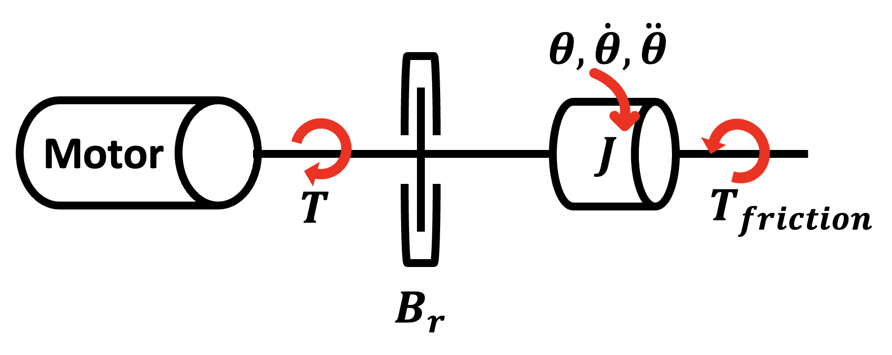
The rotational dynamics are described by:

\[J\ddot{\theta} + B_r\dot{\theta} = T - T_{\text{friction}}\]

Where \(\ddot{\theta}\) is the angular acceleration, \(\dot{\theta}\) is the angular velocity, and \(T_{\text{friction}}\) is the frictional torque opposing motion.

For a leadscrew, the frictional torque can be expressed as:

\[T_{\text{friction}} = \frac{F \cdot p}{2\pi \eta}\]

This equation demonstrates how axial force (\(F\)) and leadscrew characteristics (\(p\) and \(\eta\)) contribute to friction torque. For a detailed derivation, refer to the Appendix I.

2. Translational Equation of Motion:

The linear motion of the load is described by:

\[m\ddot{x} + b_t\dot{x} + kx = F\]

Where \(\ddot{x}\) is the linear acceleration, \(\dot{x}\) is the linear velocity, and \(kx\) represents any restoring force due to system stiffness.

3. Relationship Between Rotational and Translational Motion:

The connection between rotational and linear motion is captured by:

\[x = \frac{p \theta}{2\pi}\]

This equation relates angular displacement (\(\theta\)) to linear displacement (\(x\)). From this, we can derive velocity and acceleration relationships:

\[\dot{x} = \frac{p \dot{\theta}}{2\pi}\] \[\ddot{x} = \frac{p \ddot{\theta}}{2\pi}\]

III. Combined Equation of Motion

By combining these equations, we can express the system’s behavior in both rotational and linear domains. For a detailed derivation, refer to the Appendix II.

1. In terms of angular displacement (\(\theta\)):

\[\left(J + \frac{mp^2}{(2\pi)^2 \eta}\right)\ddot{\theta} + \left(B_r + \frac{b_t p^2}{(2\pi)^2 \eta}\right)\dot{\theta} + \frac{k p^2}{(2\pi)^2 \eta} \theta = T\]

2. In terms of linear displacement (\(x\)):

\[\left(J + \frac{mp^2}{(2\pi)^2 \eta}\right)\ddot{x} + \left(B_r + \frac{b_t p^2}{(2\pi)^2 \eta}\right)\dot{x} + \frac{k p^2}{(2\pi)^2 \eta} x = \frac{pT}{2\pi}\]

Appendix

I. Derivation of Frictional Torque in a Leadscrew

The equation for frictional torque (\(T_{\text{friction}}\)) in a leadscrew system relates the axial force \(F\) applied to the load, the pitch of the leadscrew \(p\), and the efficiency \(\eta\) of the leadscrew. Let’s break down this derivation step by step:

1. Axial Force and Linear Motion

In a leadscrew system, the axial force \(F\) applied to the load results in linear motion along the screw’s axis. The pitch \(p\) represents the linear distance the nut moves for one complete rotation of the screw.

2. Work-Energy Relationship

To understand the frictional torque, we need to consider the work done in the system:

• Work done by torque (rotational): \(W_T = T \cdot 2\pi\) (where \(2\pi\) represents one full rotation in radians)

• Work done by force (linear): \(W_F = F \cdot p\) (where \(p\) is the linear distance moved in one rotation)

3. Efficiency Consideration

The efficiency \(\eta\) accounts for energy losses due to friction and other factors. It’s defined as the ratio of useful work output to input work:

\[\eta = \frac{\text{Work Output}}{\text{Work Input}} = \frac{W_F}{W_T} = \frac{F \cdot p}{T_{\text{input}} \cdot 2\pi}\]

Rearranging this equation, we can express the input torque needed:

\[T_{\text{input}} = \frac{F \cdot p}{2\pi \eta}\]

4. Frictional Torque

In the context of a leadscrew, the frictional torque \(T_{\text{friction}}\) represents the torque required to overcome system friction and generate the necessary axial force \(F\). This is equivalent to the efficiency-adjusted input torque:

\[T_{\text{friction}} = \frac{F \cdot p}{2\pi \eta}\]

II. Derivation of Combined Equation of Motion

1. Substitution into Translational Equation

We begin by substituting the expressions for \(x\), \(\dot{x}\), and \(\ddot{x}\) into the translational equation of motion:

\[m \ddot{x} + b_t \dot{x} + kx = F\]

Substituting \(x = \frac{p \theta}{2\pi}\), \(\dot{x} = \frac{p \dot{\theta}}{2\pi}\), and \(\ddot{x} = \frac{p \ddot{\theta}}{2\pi}\):

\[m \left(\frac{p \ddot{\theta}}{2\pi}\right) + b_t \left(\frac{p \dot{\theta}}{2\pi}\right) + k \left(\frac{p \theta}{2\pi}\right) = F\]

Simplifying:

\[\frac{mp \ddot{\theta}}{2\pi} + \frac{b_t p \dot{\theta}}{2\pi} + \frac{kp \theta}{2\pi} = F\]

2. Incorporating Frictional Torque

Next, we substitute the expression for \(F\) into the rotational equation of motion:

\[J\ddot{\theta} + B_r\dot{\theta} = T - T_{\text{friction}}\]

Recalling that \(T_{\text{friction}} = \frac{F \cdot p}{2\pi \eta}\), we get:

\[J\ddot{\theta} + B_r\dot{\theta} = T - \frac{F \cdot p}{2\pi \eta}\]

Now, substituting the expression for \(F\) from step 1:

\[J\ddot{\theta} + B_r\dot{\theta} = T - \frac{p}{2\pi \eta} \left(\frac{mp \ddot{\theta}}{2\pi} + \frac{b_t p \dot{\theta}}{2\pi} + \frac{kp \theta}{2\pi}\right)\]

3. Combining and Simplifying

Grouping terms:

\[\left(J + \frac{mp^2}{(2\pi)^2 \eta}\right)\ddot{\theta} + \left(B_r + \frac{b_t p^2}{(2\pi)^2 \eta}\right)\dot{\theta} + \frac{k p^2}{(2\pi)^2 \eta} \theta = T\]

Using the relationship \(x = \frac{p \theta}{2\pi}\), we derive:

\[\left(J + \frac{mp^2}{(2\pi)^2 \eta}\right)\ddot{x} + \left(B_r + \frac{b_t p^2}{(2\pi)^2 \eta}\right)\dot{x} + \frac{k p^2}{(2\pi)^2 \eta} x = \frac{pT}{2\pi}\]