[Controller Design] Day9: Model Predictive Control - Linearization & Euler Discretization
I. Introduction
Model Predictive Control (MPC) has emerged as a powerful and sophisticated control technique, particularly valuable in industries dealing with complex, multivariable processes. Its ability to handle system constraints explicitly while optimizing control performance makes it an indispensable tool for modern control engineers.
1. Principles of MPC
MPC operates on several key principles:
a) System Model
At the core of MPC is a dynamic model of the process, typically represented in discrete-time state-space form:
\[x_{k+1} = f(x_k, u_k) \tag{1}\] \[y_k = h(x_k) \tag{2}\]where \(x_k\) is the state vector, \(u_k\) is the control input, \(y_k\) is the output, and \(k\) represents the current discrete time step.
b) Prediction Horizon
MPC predicts the system’s future behavior over a finite horizon \(N\):
\[\hat{x}_{k+i\mid k}, \quad i = 1, ..., N \tag{3}\]where \(\hat{x}_{k+i\mid k}\) is the predicted state \(i\) steps ahead, based on information available at time \(k\).
c) Control Horizon
The control horizon \((M)\) defines the number of future control moves computed:
\[u_{k+i\mid k}, \quad i = 0, ..., M-1 \tag{4}\]where \(M \leq N\). After \(M\) steps, the control input is often assumed to remain constant:
\[u_{k+i\mid k} = u_{k+M-1\mid k}, \quad i = M, ..., N-1 \tag{5}\]d) Cost Function
The control objective is formulated as a cost function to be minimized:
\[J = \sum_{i=1}^N \left\|x_{k+i\mid k} - x_{ref}\right\|_Q^2 + \sum_{i=0}^{N-1} \left\|u_{k+i\mid k}\right\|_R^2 \tag{6}\]where \(Q\) and \(R\) are weighting matrices, and \(x_{ref}\) is the reference state.
e) Optimization
At each time step, MPC solves an optimization problem to find the optimal sequence of control inputs that minimizes the cost function:
\[\min_{u_{k\mid k}, ..., u_{k+M-1\mid k}} J(x_k, u_k) \tag{7}\]subject to the constraints:
\[x_{k+i+1\mid k} = f(x_{k+i\mid k}, u_{k+i\mid k}), \quad i = 0, ..., N-1 \tag{8}\] \[y_{k+i\mid k} = h(x_{k+i\mid k}), \quad i = 1, ..., N \tag{9}\] \[x_{min} \leq x_{k+i\mid k} \leq x_{max}, \quad i = 1, ..., N \tag{10}\] \[u_{min} \leq u_{k+i\mid k} \leq u_{max}, \quad i = 0, ..., M-1 \tag{11}\]f) Receding Horizon Strategy
Only the first control input of the optimal sequence is applied, and the process is repeated at each time step.
2. Advantages and Limitations
a) Advantages
- Handles multi-input, multi-output (MIMO) systems naturally
- Explicitly incorporates system constraints in the control formulation
- Allows for the optimization of the current timeslot while keeping future timeslots in account
- Can be used to control a great variety of processes, including those with non-minimum phase, long delay or unstable processes
b) Limitations
- Computational complexity: Requires solving an optimization problem at each time step
- Model dependence: Performance heavily relies on the accuracy of the process model
- Tuning complexity: Proper selection of prediction horizon, control horizon, and weighting matrices is crucial for good performance
- Stability and feasibility issues may arise if not properly designed
3. Applications
MPC finds wide application in fields requiring optimal control under constraints:
- Process industries: Chemical plants, oil refineries, food processing
- Automotive: Engine control, adaptive cruise control
- Aerospace: Flight control systems, spacecraft trajectory optimization
- Power systems: Energy management, microgrid control
- Robotics: Path planning, motion control
- Building automation: HVAC systems, energy-efficient control
In the following sections, we will delve deeper into the mathematical formulation, implementation strategies, and advanced topics in MPC, providing you with a comprehensive understanding of this powerful control technique.
II. Mathematical Modeling and Analysis
1. Approaches for Nonlinear MPC
When implementing MPC for nonlinear systems in Simulink, especially without using iterative optimization, we can consider the following approaches:
- True Nonlinear MPC Methods:
- Multiple Shooting: Divides prediction horizon into subintervals, solving smaller optimization problems.
- Collocation Methods: Approximates state trajectories using polynomial interpolation.
- Nonlinear Programming (NLP): Directly solves the nonlinear optimization problem.
- Linearization-Based Approaches:
- Successive Linearization: Iteratively linearizes the system around the current operating point.
- Linear Time-Varying (LTV) MPC: Uses time-varying linear models to approximate the nonlinear system.
- Discretization Methods for Nonlinear Dynamics:
- Euler Discretization: Simple, fast, but less accurate for large time steps.
- Runge-Kutta Methods: Higher accuracy but more computationally expensive.
- Zero-Order Hold (ZOH): Assumes constant input over the sampling period.
- Optimization Methods for NMPC:
- Sequential Quadratic Programming (SQP): Iteratively solves a sequence of quadratic programming subproblems.
- Interior Point Methods: Transforms constrained optimization problem into a sequence of unconstrained problems.
- Genetic Algorithms: Evolutionary approach to optimization, suitable for non-smooth problems.
- Particle Swarm Optimization: Population-based stochastic technique for global optimization.
In this implementation, we will focus on trying the following approaches:
- LTV MPC with Augmented State-Space Model (Linearization + Euler Discretization)
- Linearize the nonlinear system using Jacobian linearization around an operating point or trajectory.
- Discretize the linearized system using Euler Discretization.
- Construct the augmented state-space model.
- Solve the optimization problem using Quadratic Programming (QP).
- Nonlinear Model with Euler Discretization (Direct Nonlinear Discretization)
- Discretize the original nonlinear model using Euler Discretization without linearization.
- Use this discretized model in the control algorithm.
- Solve the optimization problem using Sequential Quadratic Programming (SQP).
- Built-In Nonlinear MPC (Direct Nonlinear MPC)
- Utilize a built-in nonlinear MPC block that directly handles nonlinear dynamics.
- The built-in block manages discretization, optimization, and constraint handling.
The choice of optimization methods (QP for method 1 and SQP for method 2) is based on the nature of the resulting optimization problems. In the LTV MPC approach, linearization results in a convex optimization problem with a quadratic cost function and linear constraints, which is efficiently solvable using QP. For the nonlinear model approach, the optimization problem remains nonlinear and potentially non-convex, requiring SQP, which iteratively solves a series of QP subproblems to handle the nonlinearities.
2. LTV Linearization with Augmented State-Space Model
Now, let’s dive into one of the most practical approaches for implementing MPC for nonlinear systems in Simulink: LTV Linearization with Augmented State-Space Model. This method strikes a balance between computational efficiency and model accuracy, making it a popular choice for many control engineers. As we explore this approach, we’ll look at its advantages and potential drawbacks, helping you decide if it’s the right fit for your specific control problem.
- Advantages:
- Computational Efficiency: The linearized model reduces the complexity of the optimization problem, making QP solvers fast and suitable for real-time applications.
- Simplicity: Well-understood mathematical framework, leveraging linear algebra and convex optimization.
- Robustness: Easier to analyze stability and robustness, especially around the linearization point.
- Disadvantages:
- Accuracy: The linearization is only accurate near the operating point. If the system deviates significantly from this point, the linear model may no longer be valid, leading to suboptimal or even unstable control.
- Modeling Effort: Requires careful selection of the linearization points and may require re-linearization if the system operates over a wide range of conditions.
- Constraints Handling: While linear constraints are straightforward, nonlinear constraints require additional approximations or complexities.
- Convergence Issues:
- Local Convergence: QP solvers generally guarantee convergence to a global minimum for convex problems, which is typically the case in linear MPC. However, if the system is significantly nonlinear, the linearized model used in the QP might not accurately represent the true system dynamics, leading to suboptimal solutions or even failure to converge.
- Feasibility: If the constraints are too restrictive or the system is heavily constrained, the solver might struggle to find a feasible solution. This can lead to infeasibility issues, where the QP problem has no solution, causing the control algorithm to fail.
a) Nonlinear State-Space Model
Let’s visit Equation 13 through 17 in Day 8:
\[\begin{align*} \ddot{x} &= f_x(q, \dot{q}) + g_x(q)u \tag{12} \\ \ddot{\theta} &= f_{\theta}(q, \dot{q}) + g_{\theta}(q)u \tag{13} \end{align*}\]Where:
\[\begin{align*} f_x(q, \dot{q}) &= \frac{m_1\sin\theta(3g\cos\theta - 2l_1\dot{\theta}^2)}{4m_0 + 4m_1 - 3m_1\cos^2\theta} \tag{14} \\ g_x(q) &= \frac{4}{4m_0 + 4m_1 - 3m_1\cos^2\theta} \tag{15} \\ f_{\theta}(q, \dot{q}) &= \frac{3\sin\theta(2gm_0 + 2gm_1 - l_1m_1\cos\theta\cdot\dot{\theta}^2)}{l_1(4m_0 + 4m_1 - 3m_1\cos^2\theta)} \tag{16} \\ g_{\theta}(q) &= \frac{6\cos\theta}{l_1(4m_0 + 4m_1 - 3m_1\cos^2\theta)} \tag{17} \end{align*}\]Define state variables: \(x_1 = x\), \(x_2 = \theta\), \(x_3 = \dot{x}\), \(x_4 = \dot{\theta}\)
State-space representation:
\[\dot{x} = f(x, u) = \begin{bmatrix} x_3 \\ x_4 \\ f_x(x) + g_x(x)u \\ f_{\theta}(x) + g_{\theta}(x)u \end{bmatrix} \tag{18}\]b) Jacobian Linearization
Linearize the system at each time step:
\[\dot{x} = Ax + Bu \tag{19}\] \[A = \frac{\partial f}{\partial x} = \begin{bmatrix} 0 & 0 & 1 & 0 \\ 0 & 0 & 0 & 1 \\ \frac{\partial f_x}{\partial x_1} & \frac{\partial f_x}{\partial x_2} & \frac{\partial f_x}{\partial x_3} & \frac{\partial f_x}{\partial x_4} \\ \frac{\partial f_{\theta}}{\partial x_1} & \frac{\partial f_{\theta}}{\partial x_2} & \frac{\partial f_{\theta}}{\partial x_3} & \frac{\partial f_{\theta}}{\partial x_4} \end{bmatrix}, B = \frac{\partial f}{\partial u} = \begin{bmatrix} 0 \\ 0 \\ g_x(x) \\ g_{\theta}(x) \end{bmatrix} \tag{20}\]c) Euler Discretization
To discretize our linearized system using Euler discretization, we apply the following general formula:
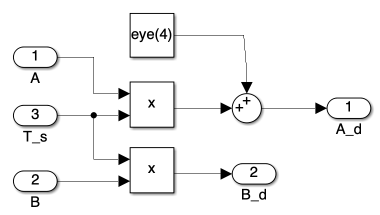
\[\begin{align*} x_{k+1} &= x_k + T_s\dot{x}_k \\ &= x_k + T_s(Ax_k + Bu_k) \\ &= (we + T_sA)x_k + T_sBu_k \end{align*} \tag{21}\]where \(we\) is the 4x4 identity matrix, \(T_s\) is the sampling time, \(x_k\) is the state vector, and \(A\) and \(B\) are the linearized system matrices as defined in Equation 19.
d) Augmented State-Space Model
Let \(A_d = we + T_sA\), \(B_d = T_sB\), \(C_d = C\) and \(D_d = D\). The system will be:
\[x_{k+1} = A_dx_k + B_du_k \tag{22}\] \[y = C_dx_k + D_du_k \tag{23}\]To improve control performance and achieve offset-free tracking, we often use an augmented state-space model. This involves including the integral action by introducing state and control increments:
\[\Delta x_k = x_k - x_{k-1} \tag{24}\] \[\Delta u_k = u_k - u_{k-1} \tag{25}\]The augmented state vector becomes:
\[x_a(k) = \begin{bmatrix} \Delta x(k) \\ y(k) \end{bmatrix} \tag{26}\]For a linear system, the augmented state-space model can be written as:
\[x_a(k+1) = A_a x_a(k) + B_a \Delta u_k \tag{27}\] \[y(k) = C_a x_a(k) \tag{28}\]where:
\[A_a = \begin{bmatrix} A_d & 0 \\ C_dA_d & we \end{bmatrix}, \quad B_a = \begin{bmatrix} B_d \\ C_dB_d \end{bmatrix}, \quad C_a = \begin{bmatrix} 0 & we \end{bmatrix} \tag{29}\]This augmented model allows for zero-steady-state error and improved disturbance rejection.
e) Prediction Model
Using the augmented state-space model, MPC predicts the future states and outputs over the prediction horizon:
\[\hat{x}_{a,k+i+1\mid k} = A_a \hat{x}_{a,k+i\mid k} + B_a \Delta u_{k+i\mid k}, \quad i = 0, ..., N-1 \tag{30}\] \[\hat{y}_{k+i\mid k} = C_a \hat{x}_{a,k+i\mid k}, \quad i = 1, ..., N \tag{31}\]where \(\hat{x}_{a,k\mid k} = x_{a,k}\) (the current augmented state). These predictions can be compactly expressed in terms of the current state and future control increments:
\[\hat{Y} = F x_{a,k} + \Phi \Delta U \tag{32}\]where \(\hat{Y} = [\hat{y}_{k+1\mid k}^T, ..., \hat{y}_{k+N\mid k}^T]^T\), \(\Delta U = [\Delta u_{k\mid k}^T, ..., \Delta u_{k+M-1\mid k}^T]^T\), and \(F\) and \(\Phi\) are defined as:
\[F = \begin{bmatrix} C_a A_a \\ C_a A_a^2 \\ \vdots \\ C_a A_a^N \end{bmatrix} \tag{33}\] \[\Phi = \begin{bmatrix} C_a B_a & 0 & 0 & \cdots & 0 \\ C_a A_a B_a & C_a B_a & 0 & \cdots & 0 \\ C_a A_a^2 B_a & C_a A_a B_a & C_a B_a & \cdots & 0 \\ \vdots & \vdots & \vdots & \ddots & \vdots \\ C_a A_a^{N-1} B_a & C_a A_a^{N-2} B_a & C_a A_a^{N-3} B_a & \cdots & C_a A_a^{N-M} B_a \end{bmatrix} \tag{34}\]Here, \(F\) represents the free response (the system’s behavior without any future control changes), and \(\Phi\) represents the forced response (the system’s response to future control increments). This formulation allows for efficient computation of predictions and forms the basis for the optimization problem in MPC.
f) Cost Function
The control objective is formulated as a cost function to be minimized:
\[J = \sum_{i=1}^N \left\|\hat{y}_{k+i\mid k} - r_{k+i}\right\|_Q^2 + \sum_{i=0}^{M-1} \left\|\Delta u_{k+i\mid k}\right\|_R^2 \tag{35}\]where \(Q\) and \(R\) are weighting matrices, and \(r_{k+i}\) is the reference trajectory.
g) Optimal Control Calculation
To find the optimal control input increment sequence, we need to minimize the cost function subject to the constraints. For a quadratic cost function with linear constraints, this becomes a Quadratic Programming (QP) problem. The unconstrained solution can be derived analytically:
First, we define the block diagonal weighting matrices:
\[\bar{Q} = \begin{bmatrix} Q & 0 & \cdots & 0 \\ 0 & Q & \cdots & 0 \\ \vdots & \vdots & \ddots & \vdots \\ 0 & 0 & \cdots & Q \end{bmatrix} \tag{36}\] \[\bar{R} = \begin{bmatrix} R & 0 & \cdots & 0 \\ 0 & R & \cdots & 0 \\ \vdots & \vdots & \ddots & \vdots \\ 0 & 0 & \cdots & R \end{bmatrix} \tag{37}\]Where \(\bar{Q}\) is an \(Nn_y \times Nn_y\) matrix (with \(n_y\) being the number of outputs and \(N\) the prediction horizon), and \(\bar{R}\) is an \(Mn_u \times Mn_u\) matrix (with \(n_u\) being the number of inputs and \(M\) the control horizon).
We also define the reference trajectory vector:
\[R_{ref} = [r_{k+1}^T, r_{k+2}^T, \ldots, r_{k+N}^T]^T \tag{38}\]Where \(r_{k+i}\) is the reference (setpoint) for the system output at the \(i\)-th step of the prediction horizon.
Now, we express the cost function in matrix form:
\[J = (\hat{Y} - R_{ref})^T \bar{Q} (\hat{Y} - R_{ref}) + \Delta U^T \bar{R} \Delta U \tag{39}\]Substituting the prediction model \(\hat{Y} = F x_{a,k} + \Phi \Delta U\) into the cost function:
\[J = (F x_{a,k} + \Phi \Delta U - R_{ref})^T \bar{Q} (F x_{a,k} + \Phi \Delta U - R_{ref}) + \Delta U^T \bar{R} \Delta U \tag{40}\]To minimize \(J\), we take its derivative with respect to \(\Delta U\) and set it to zero:
\[\frac{\partial J}{\partial \Delta U} = 2(\Phi^T \bar{Q} \Phi + \bar{R})\Delta U + 2\Phi^T \bar{Q}(F x_{a,k} - R_{ref}) = 0 \tag{41}\]Solving for \(\Delta U\) gives the optimal control increment sequence:
\[\Delta U = -(\Phi^T \bar{Q} \Phi + \bar{R})^{-1} \Phi^T \bar{Q}(F x_{a,k} - R_{ref}) \tag{42}\]In practice, only the first element of \(\Delta U\) is applied:
\[\Delta u_k = [\begin{matrix} we & 0 & \cdots & 0 \end{matrix}] \Delta U \tag{43}\]III. Simulink Implementation
In this section, we’ll explore the implementation of LTV MPC in Simulink. We’ll examine each component of our controller, explaining its purpose and implementation.
1. Overall System
The fundamental structure of the overall system, including the input/output and plant blocks, remains consistent with the model presented in Day 8.
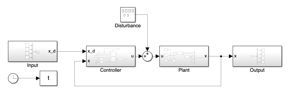
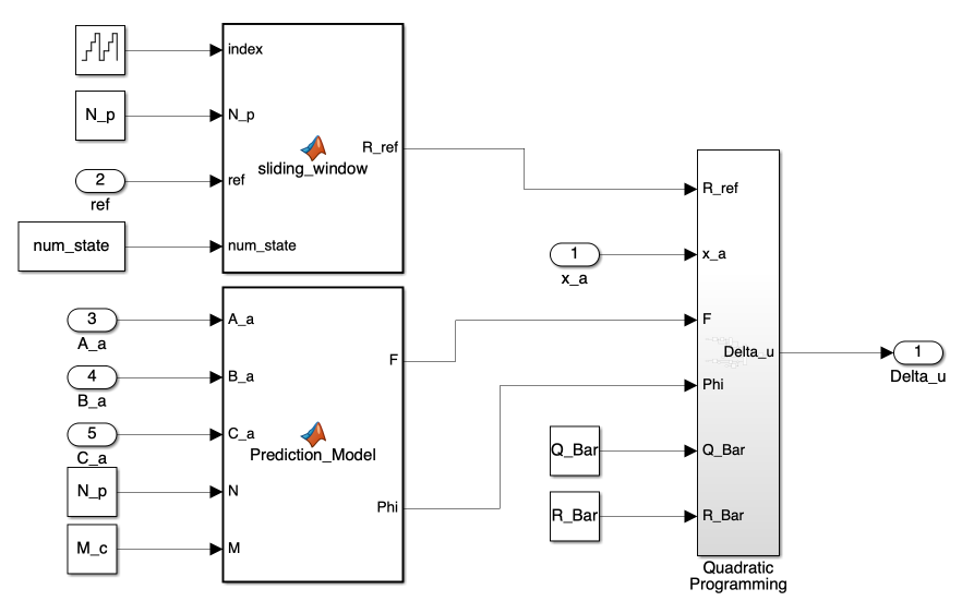
2. Controller Block
Figure 2 presents the block diagram of the LTV MPC implementation. Our controller block consists of four main processes, each crucial for implementing LTV MPC:
- Linearization
- Discretization
- State Augmentation
- Optimal Control Input Calculation
Let’s examine each of these components:
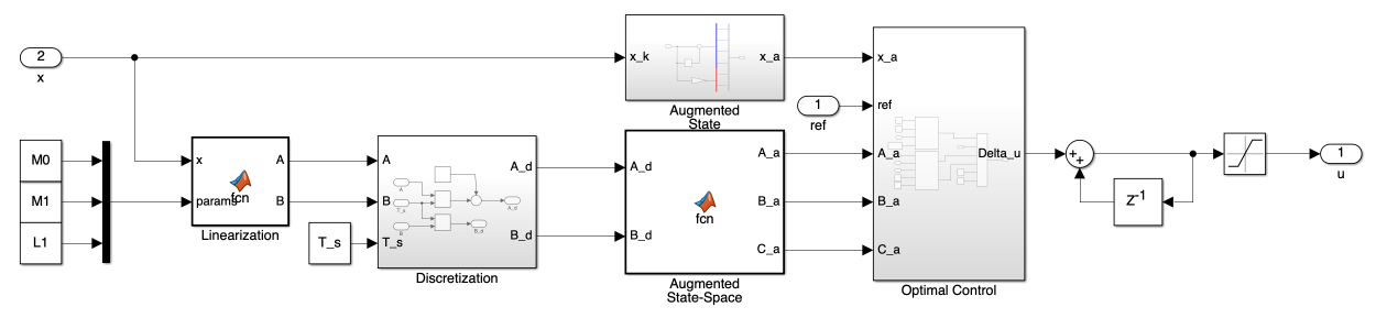
a) Linearization Block
The Linearization Block applies Jacobian linearization to the system. This block calculates the A and B matrices of our linearized system as per Equation 20.
function [A, B] = fcn(x, params)
x1 = x(1);
x2 = x(2);
x3 = x(3);
x4 = x(4);

m0 = params(1);
m1 = params(2);
l1 = params(3);

g = 9.81;

A = [0, 0, 1, 0;
     0, 0, 0, 1;
     0, (m1*cos(x2)*(3*g*cos(x2) - 2*l1*x4^2))/(4*m0 + 4*m1 - 3*m1*cos(x2)^2) - (3*g*m1*sin(x2)^2)/(4*m0 + 4*m1 - 3*m1*cos(x2)^2) - (6*m1^2*cos(x2)*sin(x2)^2*(3*g*cos(x2) - 2*l1*x4^2))/(4*m0 + 4*m1 - 3*m1*cos(x2)^2)^2, 0, -(4*l1*m1*sin(x2)*x4)/(4*m0 + 4*m1 - 3*m1*cos(x2)^2);
     0, (3*m1*sin(x2)^2*x4^2)/(4*m0 + 4*m1 - 3*m1*cos(x2)^2) + (3*cos(x2)*(2*g*m0 + 2*g*m1 - l1*m1*cos(x2)*x4^2))/(l1*(4*m0 + 4*m1 - 3*m1*cos(x2)^2)) - (18*m1*cos(x2)*sin(x2)^2*(2*g*m0 + 2*g*m1 - l1*m1*cos(x2)*x4^2))/(l1*(4*m0 + 4*m1 - 3*m1*cos(x2)^2)^2), 0, -(6*m1*cos(x2)*sin(x2)*x4)/(4*m0 + 4*m1 - 3*m1*cos(x2)^2)];

B = [0;
     0;
     4/(4*m0 + 4*m1 - 3*m1*cos(x2)^2);
     (6*cos(x2))/(4*l1*m0 + 4*l1*m1 - 3*l1*m1*cos(x2)^2)];
end
b) Discretization Block
The Discretization Block implements Equation 21. This block transforms our continuous-time linear system into a discrete-time system.
c) State Augmentation Block
Figure 4 displays the creation of the augmented state vector, Equation 26, while the MATLAB function generates the augmented state-space model, Equation 29.
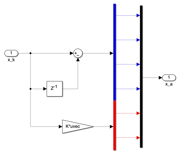
The gain \(K\) in this block represents our output matrix \(C\):
\[C = \begin{bmatrix}1 & 0 & 0 & 0 \\ 0 & 1 & 0 & 0\end{bmatrix}\]function [A_a, B_a, C_a] = fcn(A_d, B_d)
C_d = eye(2, 4);
[m, n] = size(C_d);
[~, o] = size(B_d);
A_a = eye(m+n, m+n);
A_a(1:n ,1:n) = A_d;
A_a(n+1:n+m, 1:n) = C_d*A_d;
B_a = zeros(n+m, o);
B_a(1:n, :) = B_d;
B_a(n+1:n+m, :) = C_d*B_d;
C_a = zeros(m, n+m);
C_a(:, n+1:n+m) = eye(m, m);
end
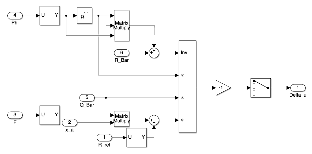
d) Optimal Control Input Calculation Block
This block consists of three main sub-blocks, as shown in Figure 5.
-
Sliding Window: This sub-block generates the reference output. As MPC assumes knowledge of the trajectory, we slide the trajectory to create \(R_{ref}\).
function R_ref = sliding_window(index, N_p, ref, num_state) index = index + 1; % x = zeros(2, N_p); x = zeros(num_state, 1000/num_state); x(:, 1:N_p) = ref(:, index:index+N_p-1); R_ref = reshape(x, 1000, 1); end -
Prediction Model: This sub-block generates F and \(\Phi\), which are used for the optimal control calculation.
function [F, Phi] = Prediction_Model(A_a, B_a, C_a, N, M) [m_A, n_A] = size(A_a); [m_C, n_C] = size(C_a); % F = zeros(N*m_C, n_A); % h = zeros(N*m_C, n_A); F = zeros(1000, 6); h = zeros(1000, 6); F(1:2, :) = C_a*A_a; h(1:2, :) = C_a; for i = 2 : N F(i*2-1:i*2, :) = F((i-1)*2-1:(i-1)*2,:)*A_a; h(i*2-1:i*2, :) = h((i-1)*2-1:(i-1)*2,:)*A_a; end v = h * B_a; % Phi = zeros(N*2, M); Phi = zeros(1000, 50); Phi(:, 1) = v; for i = 2 : M Phi(1:N*2, i) = [zeros(2*(i-1), 1); v(1:2*(N-i+1), 1)]; end -
Quadratic Programming: This sub-block represents Equation 42. It directly calculates \(\Delta U\) without constraints. For constrained optimization, the
quadprogfunction in MATLAB can be used, which is implemented in the Simulink model but not shown in this post.
Note: Instead of using \(N\) and \(M\) to create the matrices \(F\), \(\Phi\), and \(R_{ref}\), we create fixed-size matrices and use selector blocks to crop them. This approach is necessary because Simulink’s “Matrix Multiply” block cannot handle variable-size matrices.
IV. Simulation
1. Desired State vs. Trajectory (Effect of Initial Position)
To investigate the system’s behavior under different initial conditions, we examined the effect of the pendulum’s initial position. This study also aimed to compare the system’s response when using a desired end state versus a pre-generated trajectory as the control target.
a) Experimental Setup
- Initial positions tested: \(\theta_0 = 20^{\circ}\) and \(\theta_0 = 150^{\circ}\)
- Control targets:
- Desired end state \(x_d\)
- Pre-generated trajectory (using the model from Day 7)
b) Results and Observations
- For \(\theta_0 = 20^{\circ}\): The system successfully stabilized for both control targets.
- For \(\theta_0 = 150^{\circ}\): The system diverged for both the desired end state and the pre-generated trajectory.
c) Analysis
- Linearization Limitations: The system’s divergence at \(\theta_0 = 150^{\circ}\) highlights a fundamental limitation of the LTV MPC approach for highly nonlinear systems. When the initial state is far from the equilibrium point, the linearized model fails to accurately represent the true system dynamics, particularly the pendulum’s highly nonlinear behavior at large angles. This makes it challenging for the linear MPC formulation to handle extreme initial conditions.
- Control Target Comparison: Contrary to expectations, using a pre-generated trajectory did not resolve the convergence issues for large initial deviations.
Given these limitations of the LTV MPC approach for large initial deviations, subsequent simulations will focus on small perturbations around the equilibrium point to better evaluate the controller’s performance within its effective operating range.
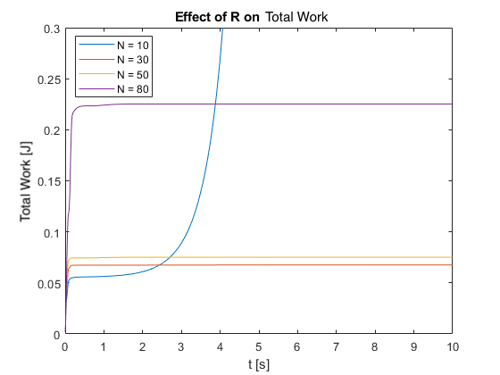
2. Effect of Varying R
To investigate the impact of the control input weighting factor \(R\) on system performance and regulation capabilities, we conducted simulations with \(R\) values ranging from 0.1 to 1000. For these simulations, we used a prediction horizon of \(N = 50\) and a control horizon of \(M = 5\). These horizons were kept constant while varying \(R\) to isolate its effects on the system’s behavior. The results are presented in the following video and figures.
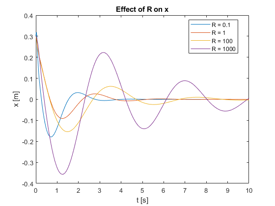
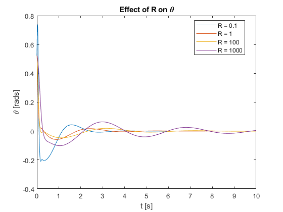
We also tested the controller’s regulation capabilities by applying a pulse force at the top of the pendulum for different R values.
a) Observations and Analysis
- Settling Time: As \(R\) increases, the settling time generally increases. This is evident in the slower approach to the setpoint for larger \(R\) values in Figures 7 and 8.
- Control Effort: Smaller \(R\) values result in more aggressive control actions, while larger \(R\) values lead to more conservative control. This is reflected in the initial rapid movements for low \(R\) values in Video 2.
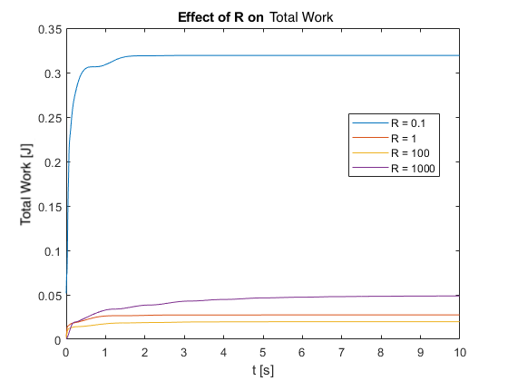
- Energy Consumption: As shown in Figure 9, energy consumption initially decreases as \(R\) increases. However, very high \(R\) values (e.g., \(R = 1000\)) can lead to increased overall energy consumption due to extended settling times.
- Overshoot: Lower \(R\) values tend to produce more overshoot, particularly visible in the \(x\) position (Figure 7) for \(R = 0.1\).
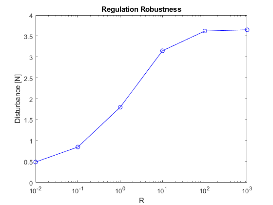
- Regulation Capability: Figure 10 demonstrates a relationship between \(R\) and the system’s ability to regulate against sudden disturbances:
- As R increases from very low values (0.01) to moderate values (10), the system’s ability to maintain stability and return to the setpoint after larger pulse forces improves significantly.
- There appears to be an optimal range (around R = 10 to 100) where the system can regulate against the largest pulse forces.
- For very high R values (>100), the regulation capability continues to improve, but at a much slower rate. This suggests diminishing returns in regulation improvement for very large \(R\) values.
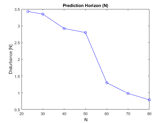
3. Effect of Prediction Horizon (N)
To investigate the impact of the prediction horizon (\(N\)) on system performance and robustness, we conducted simulations with \(N\) values ranging from 10 to 80. For these simulations, we used a fixed control input weighting factor of \(R = 1\) and a control horizon of \(M = 5\). These parameters were kept constant while varying \(N\) to isolate its effects on the system’s behavior. The results are presented in the following video and figures.
We also tested the controller’s regulation capabilities by applying a pulse force at the top of the pendulum for different N values.
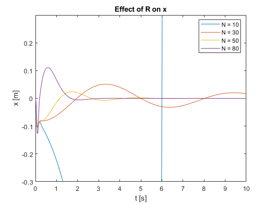
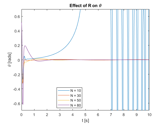
- Performance: As \(N\) increases, the overall control performance improves. This is evident in the faster settling times and reduced overshoots for larger \(N\) values in Figures 11 and 12.
- Energy Consumption: Figure 13 shows that energy consumption generally increases with \(N\). This is because longer prediction horizons allow the controller to take more aggressive actions to achieve better performance.
- Stability: Increasing \(N\) tends to improve closed-loop stability, especially noticeable for lower \(N\) values (10 to 30) in Video 3.
- Computational Load: While not directly shown in the figures, it’s important to note that larger \(N\) values increase the computational burden. In fact, very large \(N\) values (beyond 80 in this case) led to singularity issues in Simulink.
- Regulation Capability: Figure 14 demonstrates a relationship between \(N\) and the system’s ability to regulate against pulse disturbances at the pendulum top:
- As \(N\) increases, the system’s regulation capacity generally decreases. This suggests that longer prediction horizons may make the system more sensitive to sudden disturbances.
- There is a notable rapid drop in regulation capability between \(N = 50\) and \(N = 60\).
- For \(N\) values below 50, the system demonstrates better regulation against pulse disturbances.
- The decrease in regulation capability with increasing \(N\) indicates that shorter prediction horizons may be preferable for maintaining stability in the face of sudden external forces.
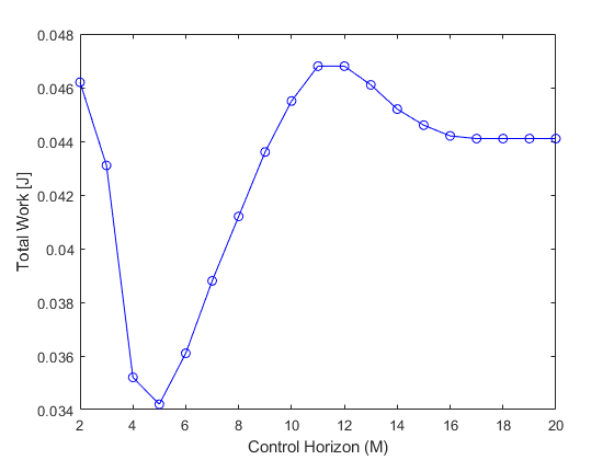
4. Effect of Control Horizon (M)
To investigate the impact of the control horizon (M) on system performance, we conducted simulations with varying M values while keeping the prediction horizon constant at N = 50 and the control input weighting factor at R = 1. The results are presented in the following video and figures.
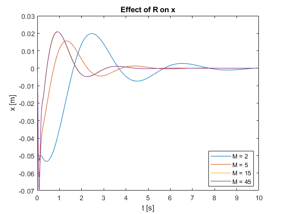
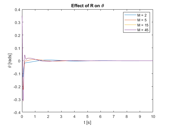
- Settling Time: As M increases, the settling time generally decreases. This is evident in Figures 15 and 16, where larger M values result in faster convergence to the setpoint for both \(x\) and \(\theta\).
- Control Effort: Larger M values lead to more aggressive control actions. This is reflected in the initial rapid movements for high M values in Video 4.
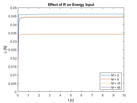
- Energy Consumption: As shown in Figures 17 and 18, the relationship between M and energy consumption is non-monotonic:
- Very small M values (M = 2) result in higher energy consumption.
- Energy consumption decreases as M increases up to a certain point (M = 5 in this case).
- Beyond this point, energy consumption increases again with M, eventually converging to a relatively constant value for large M.
- Overshoot: Higher M values tend to produce more overshoot, particularly visible in the x position (Figure 15) for larger M values.
- Robustness: While not directly measured in these simulations, it is hypothesized that very large M values might decrease system stability due to the more aggressive control inputs.
5. System Identification and Practical Performance Analysis
After tuning the control parameters, we conducted a practical performance analysis using low-frequency sinusoidal inputs to assess the system’s behavior in realistic scenarios.
a) Experimental Setup:
- Control parameters: R = 1, N = 50, M = 5
- Input trajectory: Sinusoidal with amplitude of 0.3m
- Test frequencies: 0.01, 0.05, 0.1, 0.2, 0.3, 0.4, 0.5, 0.8, 1, and 5 Hz
b) Key Observations:
- Tracking Performance: At 0.4 Hz input frequency, we observed a phase lag of approximately 0.4 seconds, indicating the system’s struggle with higher-frequency inputs.
- Frequency Response: The Bode plot reveals important system characteristics at low frequencies:
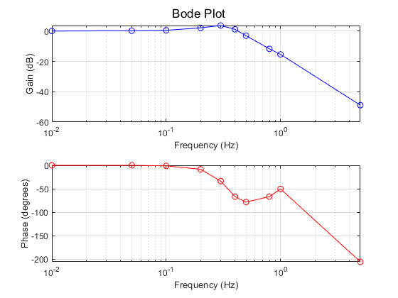
- A resonance peak was observed around 0.3 Hz, suggesting potential amplified oscillations near this frequency.
- The cut-off frequency appears to be around 0.5 Hz, indicating the system’s effective tracking range.
c) Practical Implications:
- The system performs best at frequencies below 0.1 Hz, limiting its applicability to tasks requiring slow, deliberate movements.
- Precise control becomes challenging for inputs faster than 0.4 Hz due to significant phase lag.
- The resonance around 0.3 Hz could lead to undesirable oscillations, suggesting the need to avoid sustained operation in this frequency range.
- This control setup is more suited for applications like slow-moving robotic arms or positioning systems that don’t require rapid adjustments.
IV. Conclusion
This study on Model Predictive Control (MPC) for the inverted pendulum system has provided insights into the effects of various control parameters (R, N, and M) and highlighted the inherent trade-offs in their tuning.
Key findings from our simulations include:
- Control Input Weighting Factor (R):
- Low R: Fast performance, high energy consumption, reduced stability
- High R: Slow performance, low energy consumption, improved stability
- Prediction Horizon (N):
- Low N: Reduced performance, lower energy consumption, better disturbance rejection
- High N: Improved performance, higher energy consumption, potentially reduced disturbance rejection
- Control Horizon (M):
- Low M: Slower performance, varied energy consumption (optimal at moderate M), improved stability
- High M: Faster performance, increased energy consumption, potential stability issues
- General Implications for MPC Tuning:
- Trade-offs exist between performance, energy efficiency, and stability across all parameters (R, N, and M).
- Computational complexity increases with higher N and M values, crucial for real-time implementation.
- Optimal values for R, N, and M are system-specific and depend on performance requirements.
However, our work also revealed areas for further improvement:
- Limitations of Linearization:
- The current approach relies on linearization of the nonlinear system, which is only accurate near the operating point.
- As the system moves away from the linearization point, the model’s accuracy decreases, potentially leading to suboptimal control or even instability in extreme cases.
- Absence of Constraints:
- The current implementation does not include explicit handling of system constraints, such as input saturation or state limitations.
These findings provide a foundation for understanding MPC behavior in the inverted pendulum system. To address the limitations identified in this study, our next step will be to explore nonlinear MPC techniques. This approach should help overcome the issues associated with linearization and potentially improve the controller’s performance across a wider range of operating conditions.
You can find the Simulink model on our GitHub repository.
\[\]Enjoy Reading This Article?
Here are some more articles you might like to read next: